

Application of PlanetScope-based Depth Invariant Index method in Seagrass Mapping: The study in Thi Nai Lagoon, Binh Dinh Province
- Department of Environmental Management and Informatics, University of Science, Vietnam National University - Ho Chi Minh City
Abstract
The seagrass ecosystem is one of the most critical coastal and marine ecologies. The seagrass meadows can protect the seabed coastal erosion, absorb nutrients from coastal runoff and stabilize sediments, act as bio-filters, and provide a habitat for marine animals. Nevertheless, under the impact of socio-economic growth, seagrass in the Thi Nai lagoon has disappeared and been severely deteriorated. Therefore, mapping seagrass in this area is important in informing ecologists and economists to improve sustainable marine ecosystem management strategies. This study aims to detect seagrass in Thi Nai lagoon, Vietnam, by remote sensing method. PlanetScope (PS) satellite images have high spatial (3m) resolution that is applied to extract seagrass using Lyzenga's Depth Invariance Index technique for water column correction and Maximum Likelihood Classifier (MLC). After that, evaluate the accuracy of the results using field data collected from July 29, 2020, to August 1, 2021. The study results achieved high accuracy in isolating seagrass subjects with an overall accuracy of 85.09% and Cohen's Kappa value of 0.8. There are approximately 180 hectares of seagrass in the study area. Moreover, the results also show that seagrasses are mainly distributed on the sand, muddy sand, and sandy mud along the west shore of Thi Nai lagoon and dunes such as Con Chim, Con Trang, and Con Tau, with depths ranging from 1 to 2.5 meters (90.97 %).
Introduction
Seagrasses are submerged blooming plants found in shallow coastal bays, lagoons, and along coasts1, 2. These angiosperms play a critical role in biological sediment fixing, and pollution reduction in the coastal environment. They provide refuge, incubates eggs, and habitat for fishes and small invertebrates including shrimp, crab, and other crustaceans, through their leaves and rhizomes; as the same time, they are the direct food source for herbivores or epiphytes3, 4, as well as immobilizing sediment and slow down erosion in the regions where they are found 5. In terms of pollution reduction, seagrasses absorb nutrients from coastal runoff and act as bio-filters to purify water5. Even though seagrass meadows comprise only 0.2% area of the global seabed, they have a total organic carbon content of 10-18% and annual carbon accumulation rates of 48-112 TgC/year (1teragram= 1012 grams)6. By those reasons, seagrass ecosystem services are valued at $19,000 ha-1yr-1 based on the publication of Costanza in 19977. The Thi Nai lagoon is a vast meadow of seagrasses with a remarkable diversity of species in Vietnam. However, there has been significant degradation of seagrass in this area under the impact of urban expansion, economic growth, construction of infrastructure, and aquaculture farms leading to eutrophication and the enhancement of the turbidity of the water in recent years. Therefore, seagrass mapping is essential to informing ecologists and policymakers about sustainable economic development 8.
Despite the traditional technique by field surveys obtain high accuracy and detail species level in data collection, time-consuming and wasting human labor are the two notable drawbacks of this method. To overcome these limitations, remote sensing technology has been suggested and expanded in recent decades. This approach provides impartial and truthful information on a large scale, including areas being difficult or dangerous to access9, 10, 11. Particularly, Planet (2018) observed that PlanetScope (PS) satellite can record 150 million km of Earth's surface every day. Analytic bands of PlanetScope satellite are a solar synchronous orbit with three visible bands of Red, Green, Blue, and one band of Near-Infrared Bands. Considerably, the spatial resolution of PS images is 3m while the temporal resolution is a day, which is higher than that of other satellites 12. Due to the ability to cover a wide study region and daily temporal resolution, satellite images of PlanetScope were selected as input data for establishing the seagrass map at Thi Nai lagoon.
This study aimed to contribute the approaches via remote sensing in using high-resolution satellite images to mapping seagrasses at the Thi Nai lagoon. After pre-experimental field trip for training data accumulation, the water column correction was conducted to eliminate the effect of the water column on the reflection of the substrate on the bottom boundary layer, to improve the quality of the obtained satellite images. Then the Maximum Likelihood classifier and field survey respectively occurred for seagrass detection and evaluation. This study may open up a potential method as a reference for managers and policymakers in planning and managing seagrass resources in the Thi Nai lagoon area.
Materials and methods
Study area
The objective of this study is to map seagrass in The Nai lagoon, which is one of the few areas with optimal water conditions for seagrass growth. Thi Nai lagoon is in the northeast Quy Nhon city (Nhon Ly commune, Nhon Hoi, Nhon Hai, Hai Cang ward, Thi Nai ward, Dong Da Ward, Nhon Binh ward), Tuy Phuoc district (Phuoc Son, Phuoc Thuan, Phuoc Thang, Phuoc Hoa commune) and Phu Cat district (Cat Tien and Cat Chanh communes), Binh Dinh province (Figure 1).

Map of Thi Nai lagoon in Binh Dinh province, central Vietnam.
The lagoon is between latitudes 1315’ – 1354’ N and 10912’ – 10919’ E, with a high tide area of almost 5.000 ha and a low tide area of 3.200 ha. The lagoon is connected to Quy Nhon Bay by a gate about 700m wide, and the salinity ranges from 5‰ to 32‰. The Thi Nai lagoon has brackish water due to a network of many rivers flowing into the lagoon: the Kon river and Ha Thanh River, which discharge into the top and west of the lagoon. The lagoon has a typical tropical monsoon climate (hot and humid year-round), and the water temperature in the lagoon ranging from 25C to 26.5C. The semidiurnal tide regime fluctuates from 0.4 to 2.1 meters with an average of 1.25 meters. The terrain is relatively gentle, from the top of the lagoon to the lagoon mouth.
The total area of seagrass is about 180 ha with seven species: due to the two studies of Nguyen Xuan Hoa and Cao Van Luong in 2011 and 2019 respectively 13, 14. These studies also show that the seagrass area in Thi Nai lagoon has decreased from 2003 to 2019 by 20ha. The root cause of this deterioration comes from the pressure from human activities in coastal areas.
Satellite image
The PS image used in this research was retrieved from the European Space Agency's level 3B (orthorectified scene) products (ESA) (https://www.planet.com/explorer). The image in this study was acquired on July 29, 2020 with the code numbers 20200729_022714_58_2304 and 20200729_022714_58_2304, and cloud cover was 0%, shown in Figure 5a. The radiometric resolution of the PS sceneries used in this investigation is 16 bits (i.e., 216 =65536 spectral differentiation in each pixel). It was geometrically corrected by Ground control points and fine digital elevation model resolution with a resolution ranging from 30 m to 90 m and projected to a cartographic map projection of UTM, Datum WGS84, Zone 49. Atmospheric effects were accounted by the radiation transmission code 6SV2.1. Input data for AOD, water vapor, and ozone was taken from MODIS data in near real-time15.
Data collection
Bathymetry data points were provided by the Department of Science and Technology of Binh Dinh province. After that, Arcmap 10.8 was conducted to generate a Bathymetry Map by interpolating from the depth data points using the Kriging method.
Sediment data was provided by two maps: (1) the map which was provided by the Department of Science and Technology of Binh Dinh province, and (2) the sediment map which was the outcome of the research of the author Pham Thanh Long in 2015. For the final product, Mapinfo 15.0 software was utilized to digitize the sediment map.
Field survey
The field surveys were conducted from July 29, 2020, to August 1, 2020 (Figure 1) for the purpose of training data accumulation, evaluation, and assessment. This work has referenced the studies of Nguyen Xuan Hoa (2011) and Cao Van Luong (2019) to zone the study regions.
In this study, items in aerial images were classified into four groups of seagrass, sands, sandy mud, and muddy sand, as shown in Figure 2. In order to establish important keys for seagrass distribution and bedrock detection at different depths of the Thi Nai lagoon area, boating transportation and swallow dive were performed to observe the distribution of seagrass at high tide time. Meanwhile, the point survey and quadrat method were carried out in shallow water at low tide time, as well as seagrass and other samples are also taken along the route in Phuoc Thuan, Nhon Binh commune, and Dong Da ward. As a result, more than 600 GPS points (by GPS 76CS device and iGeoTrans X Lite mobile app) were recorded to locate seagrass beds and other habitats with typical sample points. The survey sample points for each bottom habitat class were randomly divided by The Subset Features tool in Arcgis into two subsets: the training sample for the Maximum Likelihood classification and the testing sample for accuracy assessment of classification results.
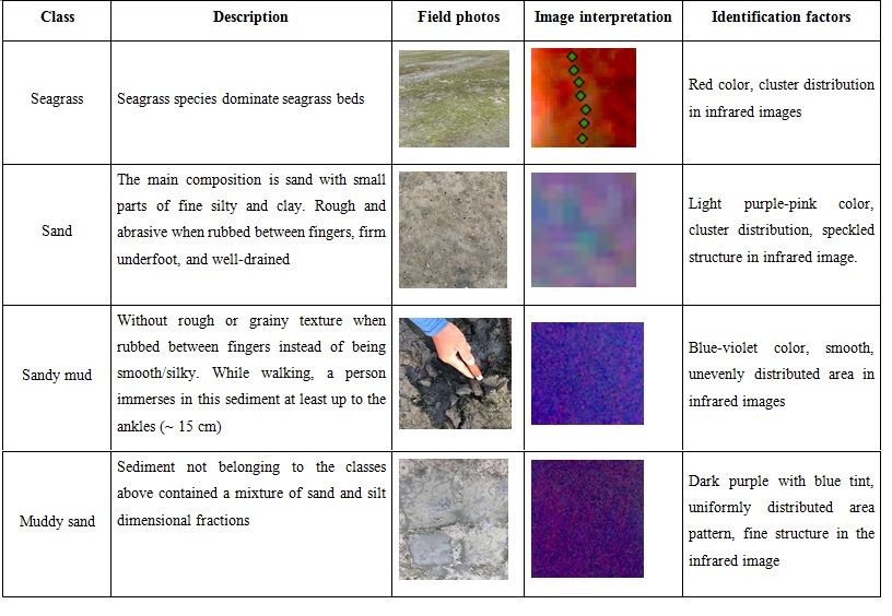
Characteristics of ground-truthing points in Thi Nai lagoon.
PlanetScope data processing for detection of the Seagrass distribution
To map seagrass by PS images, the workflow of this research is illustrated in the following Figure 3, which would be detail demonstrated in this section.

Flow chart of PlanetScope image processing for seagrass mapping.
The PS image has been corrected for atmospheric, so the next correction of the water column will be done. The Image conditions are quite clean without cloudiness and turbidity in optically shallow waters. Sun glint can be seen in deep-water areas. However, visual inspection of the RGB image in Figure 5a does not show the sun glint effect in the optically shallow water, so sun glint correction was not performed.
Before the image in the water column edition algorithm was used, PS two images had been composite, and then the composite image was cut based on the study boundary. Besides, seagrass does not appear on land. Therefore, applying the masking technique to remove noise from the mainland in the classification process is necessary.
The two main variables for applying the water column correction method are the depth value of each pixel and the knowledge of the water column attenuation characteristics. However, these variables are difficult to obtain in most fields. Thus, the water column correction method developed by Lyzenga (1981) has been used in this study because it is still effective for clear waters with several considerations such as the ease of image processing and a simple algorithm. Moreover, it does not require field measurements16.
The water column correction method of calculating DII has carried out three steps according to Lyzenga, 1981 and Mumby et al., 1998 in the Arcgis 10.8 software (Figure 4).

Water column correction procedure according to Lyzenga (1981)
Step 1: Linearing the relationship between the depth and the radiance
Xi: The transformed radiance of the pixel, calculated by the following equation (1)
Where Li is radiance at band i after atmospheric correction
Step 2: Calculating the value of ki/kj between band pairs.
According to Lyzenga in 1981, the linear equation of reflection from the bottom is based on the exponential function of bottom reflection and water depth. The dependence of Li on K, radiance, and depth is described through the equation (2):
Where: Lsi is the radiance of band i in deep water; a is a fixed value; r is the reflectance of bottom surface in band i; ki is the attenuation constant for a band i, and z is the depth from the surface to the bottom of the water.
It is impossible to follow this method because there are too many unknowns in the equation: the value of a, ki, and z. The Lygenza method18, 19 only requires the attenuation coefficients between image band pairs and does not need to calculate these parameters.
In step 2 of Figure 4, two image bands are selected, and a biplot creates each pair of spectral bands with the same substrates but at different depths. The attenuation coefficient of these bands is represented by the slope of the biplot. The gradient of the line depends on the chosen band as the dependent variable, so it is not calculated using conventional least squares regression analysis. Instead, the following equations (3), (4), and (5) are used to calculate ki/kj17.
Where: vii, vjj is the variance of band i, j, and vij is the covariance of the band i and j.
Step 3: Generating the depth-invariant index.
It is possible to obtain an index of each type of bottom substrate by recording their intercept concerning the y-axis (Figure 4 step 3). For instance, although the pixel value is on the same regression line, its brightness has changed significantly. However, they all show the same y-intercept and bottom type as sand. Since the intercept y value of seagrass pixels is different from that of sand, each bottom type's axis (or index) is called the y axis. The analytical approach carried out bases on the parametric equation of the line, shown as in equation (6):
Where: a is the regression slope, and b is the intercept of y with respect to x
Therefore, the general equation for the band pair i and j produces a band with the depth-invariant index, which is rewritten by the following equation (8):
After the water column is adjusted, the result will be used for image classification. This study used the MLC method to classify through the image classification tool of ArcGIS 10.8 software. This method is quite commonly applied in remote sensing image processing20 and taxonomists also use it in research projects of seagrass21, 22, 23. Based on training data, this algorithm assigns pixels to habitat classes using mean and covariance/variance statistics following by Benfield et al., 2007. The MLC assumes that the statistics for each class in each band are normally distributed, and the probability of a given pixel belongs to a specific class24. A statistic distance is calculated to every pixel based on mean values and covariance matrix of the clusters. Then, the pixel is assigned to the class to which has the highest probability. The Majority Filter tools smooth the image after classification in ArcGIS.
The classification results will be put into ArcGIS software to edit and calculate the seagrass cover area statistics. The map overlay spatial analysis function is used to build maps and statistics on the seagrass cover area distributed according to sediment and depth.
Using analysis errors to evaluate the accuracy of result classification is carried out by the Accuracy Assessment and Confusion Matrix tools in ArcGIS 10.825. This method in this study is based on the actual sample GPS to compare with the image interpretation results. The confusion matrix is composed of three types: Overall Accuracy (OA), User Accuracy (UA), and Producer Accuracy (PA). By the following equation9, OA represents for the number of successfully labeled pixels. Compared with field data, the UA is the probability of a pixel in the image being correctly classified. The UA is widely used because of its usefulness in assessing the classification accuracy of various habitat categories22, 26. The possibility that any pixel has been efficiently classified into each class is known as PA. Using the following equation (10), the Kappa coefficient is measured by the proportional improvement over a purely random assignment of the category 27.
Where:
N: Total number of sampling pixels, r number of class objects,
xii: the correct number of pixels in layer i,
x: total pixels in i layer of the sample, x: total pixels in i layer of the sample after classification.
The kappa coefficient is usually between 0 and 1, and for values within this range, the accuracy of the classification is acceptable. Kappa (K) has three value groups: high precision (K>0.8), moderate accuracy (0.4 < K < 0.8) and low accuracy (K<0.4)
The high accuracy of the commonly accepted classifier is above 0.85 (85%). Moderate accuracy is in the range of 0.4÷0.8. These parameters are regulated by the US Geological Survey 28.
Results
Masking image
Because the biological characteristic of seagrasses is habitat underwater, all aerial images were first applied masking techniques to remove noise from the mainland, affecting the classification process. Figure 5 depicts the framework of this process. Every RGB composite image (Figure 5a) was used to establish a binary mask image (Figure 5b) to highlight the region of interest (red color), then mask-covered images were proposed to emphasize study areas for analysis.

Example of mask technique process. (a) The RGB composite image without masking, (b) the binary mask, (c) the mask covered image.
Water column correction
In this study, we applied the water column correction technique for the corrected atmosphere images by Lyzenga's depth invariance index. This approach is implemented based on the hypothesis of the homogeneity of the bottom as well as the water environment. The sand was chosen as the substrate for the water column correction technique because it has a higher reflectance than the other substrates. The light's intensity will then decrease exponentially with depth.
Three visible bands from PlanetScope images with wavelengths ranging from 455 to 670 nm are used to generate three pairs of bands to calculate ki/kj in the process water column. Based on the relevant results of kj/ki calculations, it can obtain a pair of band that can reflect the sand value.
Linear relationships of the image band pairs can be established by natural logarithmic transformation to calculate the ratio ki/kj. The stronger the linear relationship that is, the higher the R coefficient, the more accurately the band-pair ratio will be calculated. The coefficient R for each linear equation between the channel pairs is shown in Figure 6.

Biplot of logarithmic transform bands for PlanetScope radiance images on 2020/07/29 in Thi Nai lagoon.
Figure 6 indicates that the majority of the pixel values between the bands have a linear correlation. Therefore, the image channels have correlated light attenuation as they pass through the water column. Besides, this linear correlation also emphasizes that the transformation band pair ratio pair has great accuracy.
The ratio attenuation coefficient (𝑘𝑖/𝑘𝑗) was calculated based on the variance and covariance of those bands, which outcomes into values of 0.9992, 0.9924, and 0.9941, respectively. The DIIs will be written according to the Lyzenga algorithm
Figure 7 compares the results of visual interpretation images without water column correction for the three bands ratio (RGB) of PlanetScope.

Results of visual interpretation images a) with water column correction and b) without water column correction of PlaneetScope image on 2020/07/29.
The Con Tau region, within the yellow rectangle in Figure 7, is the lagoon mouth where the runoff of the Kon River flows into the lagoon and interacts with the barrier. This creates alluvial flows and makes the water cloudy that covers seagrass meadows; therefore, the seagrass under these flows may not be detected in Figure 7a. However, after adjusting the water column, seagrasses on this dune show up in Figure 7b. By similar interpretation, the water column correction shows its essential role in the efficiency of showing the presence of seagrass meadows under alluvial flows at the region in the North of Con Chim, which is marked as red rectangles.
Seagrass classification
The RGB band ratio DII image along with more than 400 training points data was used to detect seagrass and other substrates at Thi Nai lagoon by Maximum Likelihood classification. There are four main objects selected for this labor as follows: (i) Seagrass (SG); (ii) Sand; (iii) Muddy sand, and (iv) Sandy mud. The results of this classification are shown in Figure 8.
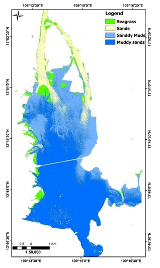
Results of the classification MLC algorithm on the DII image transformation in Thi Nai lagoon on 2020/07/29.
Confusion matrix of classification results of RGB band ratio DII
|
Class |
Seagrass |
Muddy Sand |
Sandy Mud |
Sand |
Total | ||
|
Seagrass |
102 |
5 |
3 |
5 |
115 |
88.70% |
User's accuracy |
|
Muddy Sand |
9 |
92 |
6 |
5 |
112 |
82.14% | |
|
Sandy Mud |
1 |
15 |
82 |
3 |
101 |
82.00% | |
|
Sand |
7 |
4 |
3 |
95 |
109 |
87.16% | |
|
Total |
119 |
116 |
94 |
107 |
436 | ||
|
85.71% |
79.31% |
87.23% |
88.79% |
OA = 85.09% | |||
|
Producer's accuracy |
Kappa = 0.80 | ||||||
Spatial distribution of seagrass in Thi Nai lagoon
According to the classification and application results of GIS technology, the current seagrass distribution map in the Thi Nai Lagoon area has been established (Figure 9). The total cover area of seagrass beds is estimated at 180 ha. Figure 9 figures out that seagrass beds with a large area are often concentrated in tidal flats along the west coast of the lagoon such as Dong Da Ward, Nhon Binh Ward, Phuoc Thuan Commune, and on dunes such as Con Chim, Con Trang, and Con Tau (Phuoc Son commune). Meanwhile, almost no seagrass distributes in the East, South, Southeastern, and Northernmost regions of this lagoon. The Northernmost region is the Northern mouth, where the Kon River brings alluvial deposits to Thi Nai Lagoon, this causes the high turbidity in this region, so seagrass is underdeveloped.
Figure 9a highlights that seagrasses in the Thi Nai lagoon area mainly distribute at a depth of 1 to 2.5 meters, which accounts for 163.5 ha and equivalents to 90.97% of this lagoon; while at a depth of 0.5 to 1 meter, there are 16.42 hectares (9.12%) of seagrass meadows; and notably, there are just a small amount of seagrasses which locate at the depth of 2.5 – 3 meters, only 0.16 hectares (0.09%), and this primarily belongs to Hai Minh area.
In terms of the relationship between seagrasses and the substrate on the bottom boundary layer, Figure 9b depicts that seagrasses habitat on 108.63 hectares (60.7%) of sediment in the Ha Thanh estuary area and on the dunes of the lagoon, such as South Con Chim, South Con Trang and and Con Tau; in contrast, only 10.77 hectares (6.02%) of seagrass grows on the sandy substrate of Mai Huong Lagoon and Hoi Loc Village, while 59.56 hectares (33.28%) of seagrass grows on sandy mud aquaculture ponds in shallow coastal waters.
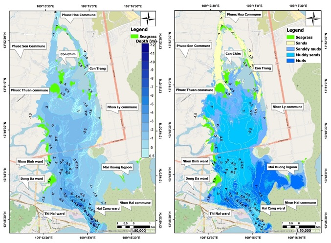
Seagrass distribution map of Thi Nai lagoon (a) overlaid with depth map (b) overlaid with sediment map on July 29th, 2020.
On the other hand, the distribution of seagrass is influenced by human activities. In the Thi Nai ward, there is a port with a very high frequency of waterway traffic, so the water here is contaminated with oil that impedes the growth of seagrass. In the East coast area of Nhon Ly commune, the results of image interpretation combined with field surveys show that seagrasses are sparse and scattered. The reason is that in these areas, sand extraction activities aim to build the project or put into shrimp ponds as well as encroach on the area to build shrimp ponds.
Discussion
The image classification results on PlanetScope are highly accurate with overall accuracy and Kappa coefficients of 85.09% and 0.8, respectively. The research results opened the potential of applying this method to other coastal lagoon areas in Vietnam, such as Phu Yen and Khanh Hoa.
The first study using PlanetScope images established the coverage of benthic habitats by Waikato et al. (2018) in the Karimunjawa Islands with an overall accuracy of 47.13–50.00% 23. Compared with this work, the present study achieves higher accuracy. It is also possible that our use of Lyzenga's 1981 water column correction contributed to the improved accuracy of our results. Therefore, using this correction method for seagrass mapping in our study area is appropriate.
In this study, the correction method of Lyzenga 1981 was used. This method has greatly supported the image interpretation of seabed types, establishing thematic maps with higher accuracy 17. So far, there have been many studies on the correction methods of the influence of water column depth on image radiation. Still, these methods are derived from the calculation method of Lyzenga8, 17. Sagawa’s new method describes the mathematical relationship between the reflectivity of the bottom surface and the radiation level measured by the sensor on the remote sensing satellite. Sagawa proposed a new index, the Bottom Reflectance Index (BRI). The results of the author Sagawa’s research not only highlight the applicability of Sagawa’s method, but also highlight the image interpretation of areas with low water transparency8. Thus, for waters with higher transparency, the Lyzenga or Sagawa method can be used. However, for waters with lower transparency, Sagawa's method is more accurate.
The depth-invariant images had a significant visual improvement, which was reflected in the classification accuracies, although the Lyzenga method is only effective in clean water19, 22. The cause for this could be due to image quality or atmospheric conditions. PlanetScope images were atmospherically corrected according to the European Space Agency's procedures and then masked to remove some noise before the water column was corrected and the images were classified in this study.
Turbidity is an important factor affecting satellite data processing and classification outputs29, 30. High turbidity causes the light intensity to decrease rapidly with depth, making seagrass detection harder. According to Jerlov in 1951, coastal waters have a stronger light attenuation than seawater 31. Therefore, it is more difficult to estimate the presence and distribution of seagrass in the Thi Nai lagoon compared to other areas. This causes the Kappa coefficient and accuracy in our study to be lower than that of Hang et al. (2019) with an OA of 88.58% and Kappa coefficient of 0.8445 at My Quang - Hon Chua, Phu Yen province, despite using the same PlanetScope image and Lyzenga correction method 32.
In addition to environmental factors and sources of satellite sensors, the interpretation process of SAV also relies on classification methods21, 33. In this study, the Maximum Likelihood Classifier (MLC) algorithm was applied to classify substrate types. However, the linear discriminant function of MLC may not work when the boundary between seagrass and other benthic habitats is not clearly defined, which may lead to misclassification between seagrass and other benthic habitats21. Machine learning (ML) is a recent technological advance that can ameliorate these limitations and is the recommended new approach for seagrass mapping in different time scales. Research results from Ha et al. (2020) have shown that the ML method is better than the MCL when comparing the MCL with Random Forest, Rotation Forest, Canonical Correlation Forest to map seagrass using Sentinel-2 images in Port Tauranga, New Zealand. Furthermore, Pham et al. (2019) also propose ML techniques for mapping coastal vegetation considering the limitations of the MLC method34. Although ML technology has several benefits, the application of this method in the field of seagrass maps is still in its infancy21, 34. Therefore, with the development of ML technology for multi-source remote sensing image application seagrass mapping, various algorithms should be encouraged for future research.
Our findings on the seagrass distribution are similar to those in the Cao (2019) report 14. Seagrass beds have a large area distributed in tidal flats along the west coast of the lagoon and on dunes such as Chim, Trang, and Tau. This may be due to the close time between the two studies; hence the distribution and area of seagrass have not changed (approximately 180 hectares). At the same time, our research results demonstrate the ability of PlaneScope images to detect submerged aquatic vegetation.
Conclusions
The distribution of seagrass beds in Thi Nai lagoon, Binh Dinh province, can be detected very well by PlanetScope satellite image. In addition, thanks to the pre-processing of data by the Lyzenga algorithm in 1981 and the masking technique in the PlanetScope image, the water column effect as well as other random noises were removed.
PlanetScope satellites acquire images near-daily; thus we can obtain remote-sensing images very close to the field date. As a result, the time deviation is minimal, contributing to improved accuracy for dynamic mapping objects. The resulting study shows that the overall accuracy and the Kappa coefficient used to evaluate the accuracy of the MLC method provide high results (OA=85.09% and Kappa=0.8).
The total seagrass area in this study is estimated to be about 180 hectares. The seagrass is mainly distributed on sand, muddy sand, and sandy mud on the west coast of Thi Nai lagoon and on dunes such as Con Chim, Con Trang, and Con Tau with the depth of 1-2.5m (90.97%).
Using remote sensing technology and geographic information system, combined with field survey data, the Thi Nai Lagoon seagrass distribution map was established. These outcomes will protect the seagrass bed and the sustainable development of Thi Nai Lagoon's aquatic resources.
List of abbreviations
DII Depth Invariant Index
ML Machine learning
MLC Maximum Likelihood Classifier
OA Overall Accuracy
PA Producer Accuracy
PS PlanetScope
UA User Accuracy
Competing interests
The authors pledge that they have no conflicting interests.
Author’s contribution
Tran Thi Thanh Dung participated in the calculation, processing and data collection and wrote the manuscript itself;
Tran Tuan Tu participated in the ideation of the article and edited the manuscript.
Acknowlegdments
We would like to thank the Planet Education and Research program for providing the opportunity to use and evaluate the performance of PlanetScope images.