Breast cancer diagnosis based on detecting lymph node metastases using deep learning

Abstract

Introduction: Automated detection of metastatic breast cancer from whole slide images of lymph nodes utilizing a deep convolutional neural network was proposed in this study.

Methods: The dataset is taken from the PatchCamelyon subset, which contains 220,025 images divided into training, validation, and testing sets at a ratio of 60:20:20. The pretrained ResNet50 model was utilized, and transfer learning was subsequently applied to adjust the weights of the model. To elevate the model performance, the evaluation metrics were assessed by the accuracy score, confusion matrix, receiver operating characteristic (ROC) curve, and area under the ROC curve (AUC) score.

Results: As a result, the proposed algorithm obtained high performance, with scores over 95% in all the evaluation methods, especially the AUC score, which achieved 0.989. Moreover, the model is validated in a testing set with the test-time augmentation (TTA) technique to enhance prediction quality and reduce generalization error.

Conclusion: Overall, the proposed model achieves high accuracy when applying transfer learning. The results prove that the trained Resnet50 model can extract useful information from small cells in histopathologic images for breast cancer detection.

Introduction

Breast cancer, which occurs when cells in the breast start to grow uncontrollably, is the leading cause of death in women and has become one of the major global public health problems. Breast cancer is straightforwardly influenced not only by the quality of life of the patient but also mentally and emotionally by the patient and by the diagnostic and therapeutic procedures. Moreover, it also indirectly affects the patient's family, marital relationship, and economic and social problems 1 . According to statistics from the National Cancer Institute, breast cancer is the most common cancer in women after skin cancer and is the second leading cause of death after lung cancer 2 . In 2019, approximately 268,600 diagnosed cases of breast cancer were reported and accounted for approximately 15.2% of all new cancer cases. Meanwhile, an estimated 41,760 deaths are caused by breast cancer (accounting for approximately 6.9% of all cancer deaths) 3 . In Vietnam, there are approximately 18 people with breast cancer every 100,000 people. It is estimated that there are approximately 11,000 new cases a year and over 5,000 deaths 4 . Recently, the death rate from breast cancer has decreased, while the incidence of this disease has not decreased. This is unlikely to be the result of advances in the prevention or screening of mammograms. In other words, advanced results in the invasive diagnosis of breast cancer to accurately determine the cancer stage and thereby improve the effectiveness of treatment 5 . Therefore, when someone is diagnosed with breast cancer, it is very important to determine if cancer has metastasized because late-stage cancer is responsible for over 90% of cancer deaths.

Breast cancer is a condition in which breast cells grow abnormally; more specifically, some malignant tumors have developed from cells in the breast. One of the causes of breast cancer is that cancer cells can grow and invade healthy breast tissue or other organs through the lymph nodes, becoming advanced stage or metastatic cancer. It is mentioned that lymph nodes are small glands that filter fluid in the lymphatic system, and they are one of the first places breast cancer spreads. If not detected early and treated promptly, breast cancer will spread to some common sites, such as lymph nodes, bones, liver, lungs, and brain; when it metastasizes to the bones and brain, the patient has to fight with tormenting pain every day. One of the methods of diagnosing breast cancer is that the pathologist examines the histology with a microscopic microscope after a biopsy or surgical sample to study the manifestations of the disease. However, these diagnostic procedures are tedious, repetitive, and time-consuming for pathologists because of having to examine large areas of tissue and easily missing small metastases 6 .

Recently, the advances and development of artificial intelligence (AI) or machine learning (ML) models have generated methodologies to help pathologists or doctors in medical diagnosis, screening in the early stage, and treatment more accurately 7 . The diverse applications of extracted modeling in cancer research have been performed and reported in many studies for early modeling of cancer risks or for rapid and accurate diagnosis of patient outcomes. In breast cancer screening, predictive models based on advanced image processing techniques and AI technology have been established for the early diagnosis of cancer outcomes. Together with the development of convolutional neural networks (CNNs), multiple CNN architectures have been generated, such as ResNet (in 2016) 8 , GoogleLeNet (in 2014) 9 , VGGNet (in 2014) 10 , AlexNet (in 2012) 11 , and Nasnet (in 2018) 12 . The architectures share the same layers’ structure but differ from the number of layers, feature mapping, and hyperparameters. Among them, Residual Neural Networks (ResNet), proposed by He et al. 8 , has the layers reformulated for learning with residual functions instead of nonreference functions. Therefore, the ResNet models are easier to optimize and gain significant accuracy from an enhancement of network depth.

Numerous methods of breast cancer diagnosis have recently been researched and developed with admirable results. An early work by Prentice and Gloeckler was published in 1978 13 on a statistical model known as the proportional hazard regression model to identify whether patients survived based on breast cancer data collected at that time. Later, in 2005, Delen and his group 14 applied artificial neural networks (ANNs), decision trees, and logistic regression to progress their predictive model of breast cancer patient survival using a published SEER dataset containing 433,272 images of 72 variables from 1973 to 2000. Their results showed that decision trees are the best predictor of all chosen models that achieved a performance of 0.9362 in the accuracy of classification. Then, in 2008, Khan et al. 15 contributed an enhancement in the prognostic model of the survivability of breast cancer patients by analyzing the combination of accuracy and interpretability with regard to fuzzy logic and decision tree models. Concurrently, Thongkam and his group 16 utilized RELIEF attributed selection to complement preprocessing and the Modest Adaboost algorithm to forecast the survivability of breast cancer patients. Their results showed that their proposed algorithm performs better than Real and Gentle AdaBoost. Recently, Dhahri et al. 17 and Naji et al. 18 used the published breast cancer dataset from Kaggle 19 to detect and classify benign and malignant tumors. The dataset provides ten features (including radius, texture, perimeter, area, smoothness, compactness, concave points, symmetric, and fractal dimension) that are extracted from a digitized image of a fine needle aspirate of a breast mass. These studies applied some traditional ML algorithms, such as support vector machine, random forest, and gradient boosting. to confirm the potential of ML applications in diagnosing breast cancer. The performance of these classifiers achieved a high accuracy of above 90%.

In addition to improvements in predicting breast cancer outcomes, detecting models have been developed to aid physicians or pathologists in diagnosing breast cancer more quickly and accurately. Feature engineering has brought some significant improvements to ML models in healthcare, especially in image analysis allowing computers to examine obvious features in images or even detect lesions and abnormal areas in the image. Therefore, the objective of this study was to develop a predictive model utilizing deep learning (DL) algorithms to detect the presence of lymph node metastases in breast cancer histopathologic images to more accurately determine the stages of breast cancer. Obviously, it is easier to classify breast cancer from a tabular dataset, as described in 17 , 18 , than from a color (histopathologic) image dataset. Therefore, the DL model is applied for binary classification in the proposed study. Moreover, some optimization techniques are also used to reduce the time-consuming training of the model and obtain high accuracy for performance. The main challenge in this study is that metastases are capable of being small in size as single cells in a large area of ​​tissue. Finally, the performance of the proposed model was examined by evaluation metrics, including the accuracy score, confusion matrix, ROC curve, and AUC score.

Material and methodology

Data preparation

Dataset

Figure 1 shows some images of the positive and negative metastasis samples of the PatchCamelyon dataset 20 collected from five different medical centers in the Netherlands. The dataset contains 220,025 images, including 89,117 samples that were labeled positive for metastases and 130,908 samples that were labeled negative. It is noted that the sample was determined positive if there was at least one pixel of metastatic tissue in the central region of 32 × 32 pixels in the image. Tumor tissue in the outer region of the image did not affect label identification. Each image has a size of 96×96 pixels in the type of color image (i.e., 3 channels) and TIF format extracted from whole slide images (WSIs) from hematoxylin and eosin-stained lymph node sections. The dataset is split into three sets for training, validation, and testing, with a portion of 60:20:20. Table 1 presents the number of samples used for the training, validation, and testing sets. It is noted that the distribution ratio of the dataset is approximately 40:60 of positive and negative (i.e., 89117:130908 images).

Figure 1 . Images of positive and negative metastases samples 20 .

Table 1 Number of samples in the training, validation, and testing sets .

Data processing

Figure 2 presents the general pipeline of the experimental model from preprocessing to evaluation. There are four main stages in the experimental process, where each stage serves as the foundation for the next stage. In the first stage, the preprocessing step is discovering the dataset to comprehend the properties and process the data before training. The data preparation step helps prepare a clean, stratified-split dataset and applies augmentation methods to prevent data leakage and overfitting by conducting statistical tasks, noise filtering, rotation, cropping or zooming of the image. The second stage is to build models to yield a set of parameters for the selected model for optimal training results. Subsequently, in the third stage, the built model is trained with selected hyperparameters to create a well-trained model. Finally, the trained model is evaluated by performance metrics, including loss score, accuracy graph, confusion matrix, receiver operating characteristic (ROC) graph, and area under the ROC curve (AUC) score.

Figure 2 . Experimental pipeline.

ResNet50 and transfer learning

Since high-performance models are usually demanding in computing, to save training resources, models were chosen with a high evaluation score in the relative size range. In this proposed study, the Resnet50 pretrained model 8 was deployed, and then transfer learning was utilized to emplace the weights of the model.

The advantage of ResNet50 is to have a deeper network and address the depth issue by training the interactions among slightly different layers. In contrast to the drafting of layers as in VGG16, ResNet50 employs residual units as "shortcut" identity connections between the layers. This system then trains the layers relative to their residuals instead of the original values. This solves the problem of loss of accuracy inherent as the networks become deeper. It is clear that ResNet50 provides the possibility for training deeper networks with a depth of up to 152 layers and further enhancing the quality of the model.

In this study, the transfer learning technique is applied by the pretrained model learned in ImageNet and the technique of fine-tuning the weights to fit the new dataset. This technique works very efficiently in practice because it allows the model to employ previously learned features, fuse and match them in new combinations, and apply to a new image set. In addition, transfer learning also exhibits superior performance compared to the method of training the model from random initialization. Specifically, the model that applies transfer learning will converge much faster and more accurately in many cases. Therefore, transfer learning not only provides enhanced prediction results but also yields a faster training process.

Performance evaluation metrics

Accuracy

Accuracy can be defined as the number of correct predictions compared to the total predictions of samples. However, it will be inefficient when the dataset is unbalanced. The dataset used in this study is quite balanced thus, the accuracy metric is appropriate. The accuracy is formulated as follows:

where TP, TN, FP, and FN are true positive, true negative, false positive, and false negative, respectively.

Confusion matrix

The confusion matrix is ​​a table with four positions corresponding to four different combinations of predicted and actual values ​​(i.e., TP, FP, TN, and FN). TP is the total of the positive predictions that are truly positive, whereas FP is the total of the positive predictions that are not truly positive. TN is the total number of negative predictions that are truly negative, while FN is the total number of negative predictions that are not truly negative.

The confusion matrix is ​​commonly used to analyze four values ​​namely, positive predictive value, negative predictive value, sensitivity, and specificity. Normally, models tend to focus on an analysis of positive predictive value (i.e., precision) and sensitivity (i.e., recall). Precision is the probability that a positive prediction is actually correct, while recall is the proportion of actual positives being identified correctly. Precision and recall can be formulated as follows:

AUC/ROC/TTA

The receiver operating characteristic (ROC) curve is a graph depicting the TP rate versus the FP rate at all thresholds. ROC evaluates the ability of detection of the binary classification system. Each point on the ROC curve illustrates a precision/recall pair corresponding to each detail threshold. Meanwhile, the area under the ROC curve (AUC) calculates the total area below the entire ROC curve from the origin position (0,0) to the position (1,1) in a two-dimensional coordinate axis. The AUC provides information on a comprehensive measuring performance across all possible classification thresholds. In other words, the AUC deputizes the probability that the model rates a random positive sample higher than a random negative sample. It is noted that a model that produces 100% of the wrong prediction has an AUC of 0.0 and that of 100% correct prediction is 1.0.

Furthermore, the proposed model is also validated by the testing set to return evaluation results (i.e., Test-time data augmentation (TTA)). TTA 21 was utilized to enhance prediction results and shorten generalization errors. Specifically, each image was predicted with different versions, and the final score was averaged from the prediction score (i.e., 5 in this study).

Hyperparameters for deep learning

To optimize the model and minimize the generalization error, several strategies have been applied for modification and optimization. Therefore, model optimization is one of the biggest challenges and requires time-consuming implementation of deep learning solutions. Deep learning models normally deal with learning rates, the number of hidden layers, and dropout rates.

Learning rate

The learning rate is a hyperparameter that manages the magnitude of the updated weights to minimize the loss function in the training process. Choosing the learning rate is a challenge, as if the learning rate is too small than the optimal value, it will consume a long time to reach the point of convergence. Conversely, if the learning rate value is too large than the optimal value, the training model might lead to learning the suboptimal weights too quickly or might not converge due to the unstable training process.

Drop-out

Drop-out 22 is a technique to prevent the overfitting of the model and concurrently to provide a way to approximately combine multiple neural networks exponentially and expeditiously. “Drop-out” mentions the drop-out units (i.e., hidden and visible) in the neutral network. This technique will temporarily ignore some units that cannot participate and contribute to the training process. Normally, choosing which units to drop is random.

Hyperparameters for transfer learning

In this proposed study, the pretrained Resnet50 model was deployed, and transfer learning was subsequently utilized to adjust the model weights. It is noted that histopathologic images are different from the images on ImageNet consequently, some specific features of the last layers were trained.

Figure 3 shows the learning rate and loss score of the proposed study. As shown, with the learning rate of 1e-4 (i.e., 0.0001) – the largest weight decay gives a low loss. Based on the One cycle policy proposed by Smith et al. 23 , it is found that 1e-4 is an acceptable learning rate.

Figure 3 . The results of learning rate and loss score.

Figure 4 . The accuracy scores of the training and validation datasets with a learning rate of 1e-3.

Figure 4 demonstrates the accuracy score of 10 epochs with a learning rate of 1e-3. It can be seen that the model tends to be underfitting when the accuracy of the validation set is much higher than the accuracy of the training process in the first epoch. It can also be observed that when the learning rate was reduced to 1e-4, the model was more stable and closely converged.

It is observed that the size of the images has a large effect on the performance of the model. Specifically, the dataset was first trained with an image size of 224 x 224 pixels, and the accuracy was 86% compared to the 95% accuracy score on the validation dataset. It is remarked that 224 x 224 pixels is the default image size of the ResNet50 architecture. To decrease the processing time by reducing the image size, the image size was reduced gradually. The results showed that 196 x 196 pixels is the most efficient size that offers both a similar accuracy score and a shorter training time compared to 224 x 224 pixels of image size.

In addition, regarding the drop-out rate, to minimize overfitting when applying the pretrained model, a 0.5 drop-out rate was set. Moreover, after tuning the hyperparameters, the training dataset was fed into the built model and trained for 10 epochs. The accuracy and loss values are then calculated for examination on the training and validation sets. Finally, the ROC and AUC curves were plotted and calculated.

Results and discussion

Training results

Figure 5 illustrates that the training loss and validation loss slowly decreased, and at the same time, the training and validation accuracy progressively increased over epochs. This means that the model is trained accurately and effectively. As shown, from epochs 7 to 10, the loss and accuracy scores are obviously stable. This proves that the model learned almost all features from data images after a few epochs when transfer learning with the optimized hyperparameters was applied.

Figure 5 . The loss and accuracy scores on the training and validation datasets.

After training the pretrained Resnet50 model with transfer learning, the best weights for the model were selected as the chosen weights obtained the lowest validation loss. Figure 6 presents the confusion matrix for evaluating the performance of the model by statistical parameters. The results showed that there were 16185 cases of true positive (TP), 25651 cases of true negative (TN), 531 cases of false positive (FP), and 1638 cases of false negative (FN).

Figure 6 . The result of the validation set.

Evaluation results

Continuously, the best candidate from the trained model based on the AUC score was put to the final test. Additionally, the model combined with the TTA technique was validated by the testing set to return evaluation results. Successively, prediction results from the model were utilized to estimate the confusion matrix, as shown in Figure 7 . This means that the proposed model correctly detected 16,980 positive cases and 25,674 negative cases, but it still classified incorrectly from negative to positive in 507 cases and from positive to negative in 844 cases.

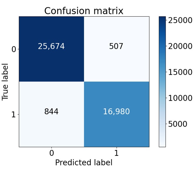
Figure 7 . Confusion matrix of the testing set.

Figure 8 shows the ROC curve result with true positive and false positive rates at different thresholds. As shown, the AUC score was estimated and was 0.989. This result demonstrates that the proposed algorithm performed well in all thresholds.

Figure 8 . ROC curve and AUC score results.

Subsequently, the confusion matrix results were deployed to estimate the performance metrics, including the precision, recall, and accuracy (see Table 2 ). The results showed that all performance metrics on the testing set were superior to those on the validation set. This is the fruitful effect of the applied TTA technique mentioned above. Moreover, these results prove the reliability of the proposed algorithm and method.

Table 2 Results of validation metrics on the validation and testing datasets.

Discussion

Generally, the proposed model has a high performance with a score of over 95% in all evaluation methods, including precision, recall, accuracy, ROC curve, and AUC score. Furthermore, the model follows the data and the original aim for automatically detecting metastatic cancer from histopathology images of the lymph nodes. One advantage is that the proposed model can work effectively with the raw data based on preprocessing, which leads to a reduction in the cost of preprocessing. Additionally, the model is established on the Keras platform with friendly and easy handling characteristics. However, the model exposed the drawback of a long training time of approximately seven hours for ten epochs of training.

Table 3 Comparison of the results of the proposed study to those of other studies

For the same solving purpose, the results from several studies are compared in Table 3 . As shown, the proposed model achieved a remarkable result with a 0.989 AUC score. Specifically, the proposed model outperformed both studies in 17 , 18 that used traditional ML algorithms with the Wisconsin-breast cancer dataset. This dataset is slightly simple, with ten real-valued features that are computed from digitized images by the authors 19 . These studies applied some techniques at the preprocessing step to reduce the number of features and dimensions of data before being fed into ML algorithms. The results in 17 also showed that their classifiers were not trained well enough for imbalanced data because of obtaining high accuracy but having a low AUC score. Naji et al. 18 presented better performance with similar ML algorithms after optimizing the hyperparameters. The selected classifiers in 18 achieved higher accuracy and AUC scores than those in 17 . The comparison between the proposed model and the studies in 17 , 18 demonstrates that the combination of the DL model with transfer learning techniques is a powerful tool for extracting useful information from large and complex datasets, such as histopathologic images. In addition, the LYNA algorithm 24 achieved the highest AUC score of 0.99. However, the Camelyon16 dataset utilized in the LYNA algorithm study is fairly small, with only 270 images with high resolution. Furthermore, their model was trained with 40X magnification data consequently, the evaluation score was very high. Instead, with the small size of the dataset as mentioned above, their model usually tends to overfit. Meanwhile, when the dataset is relatively large, the model experiences a long processing time when applying this strategy. Regarding the results of Zhou et al. (2019) 25 , training the model for the detection of metastatic lymph node cancer using ultrasound images is uncommon. The root cause is that the ultrasound image has many drawbacks, such as indistinct margins, irregular shapes, and visualized nodes only. However, with the discouraging data type, their model also contributed greatly to the advanced diagnosis of lymph node cancer based on deep learning utilization. Finally, in comparison of two Top 3 Kaggle competition models using the same dataset, the performance of the proposed model in this study outperformed the others. Specifically, on the Camelyon17 dataset, the two Top 3 Kaggle competitors and the proposed study achieved AUC scores of 0.9648, 0.9543, and 0.989, respectively. Moreover, in these two Top 3 Kaggle competitors' studies, the authors used the Fastai library, which has fast processing speed and available algorithms for hyperparameter optimization. In other words, the fine-tuned DenseNet pretrained model is a new architecture with the high ability of concatenation for creating new features that are deployed in these two studies. In particular, instead of each layer connecting to the preceding layer in other models, each layer in the DenseNet model possesses supplemental inputs from all previous layers and passes on its own feature maps to entire subsequent layers.

Obviously, it is seen that the errors generated by the model are often lower than those caused by humans. However, it is not possible to infer whether the error from the computer network and the pathologist's performance are correlated. Henceforth, in the future, this research may combine advanced deep learning algorithms and pathologist capabilities to improve model accuracy, repeatability, and reproducibility for pathological diagnosis. Furthermore, this proposed study can be extended in different aspects, including (1) optimizing hyperparameters to obtain better performance; (2) experimenting with other architectures to choose the best one; and (3) adding more up-to-date and developed models with three classes, including normal, nonmetastatic and metastatic cancer, to increase sensitivity and practical applicability for the system.

Conclusion

In this study, automated detection of metastatic cancer from lymph node images using a deep convolutional neural network was conducted and proposed. The ResNet50 pretrained model and transfer learning were utilized to adjust the weights of the proposed model. The patch Camelyon17 dataset with 220,025 images was deployed, and the training-validation-testing set ratios were 0.6, 0.2, and 0.2. As a result, the model performance was assessed by the evaluation metrics (i.e., precision, recall, and accuracy score) from the testing set, obtaining 97.10%, 95.26%, and 96.93%, respectively. Moreover, the AUC score obtained from the ROC curve was estimated to be 0.989. These outperformance scores infer that the proposed algorithm and model performed effectively in all thresholds. Finally, the proposed model is validated in a testing set with the TTA technique to enhance prediction quality and reduce generalization error.

ACKNOWLEDGMENTS

This research is funded by Vietnam National Foundation for Science and Technology Development (NAFOSTED) under grant number 103.03-2019.381.

Authorship contribution statement

Thach Nguyen Bich Ha: Methodology, Formal analysis, Investigation. Ngoc-Bich Le: Writing – original draft. Ngoc Trinh Huynh: Formal analysis, Investigation. Thanh-Hai Le: Visualization, Investigation, Data curation. Thi-Thu-Hien Pham: conceptualization, methodology, formal analysis, supervision.

Declaration of competing interest

The authors declare that they have no known competing financial interests or personal relationships that could have appeared to influence the work reported in this paper.