Sensor Rotational Measurement with Virtual Sensors Applying Pearson Generative Adversarial Imputation Nets

Abstract

Recent advances in sensor technology have increased the ability of humans to measure a wide range of phenomena and events. Nevertheless, in some cases, due to a variety of limitations, only a few sensors can be deployed at a given site. Consequently, setting up enough sensors at the right places to provide uniform monitoring can be difficult. In addition, virtual sensing, which is a set of strategies for replacing a portion of physical sensors with virtual sensors, has recently been developed. Therefore, this work leverages the imputation capability of PGAIN-VS to develop a black-box data-driven virtual sensing approach named sensor rotational measurement for the purpose of reducing the number of physical devices to be used in reality while still ensuring monitoring accuracy. The approach takes advantage of the PGAIN-VS and Borda voting methods to determine the subset of real sensors that can take turns observing information within an interval of time. The approach is seen as a black-box objective optimization problem with constraints that is solved by the OpenBox tool. We evaluated our method on several real-world datasets and achieved promising results, with the overall number of physical sensors reduced by up to 20%.

INTRODUCTION

Currently, the terms Internet of Things (IoT) and edge computing have appeared in most areas and provided many benefits for businesses as well as people’s lives because they have created many smart industries, namely, smart villages, smart homes, smart farming, and more. However, why is this the case? The answer is because the utilization of numerous different physical sensor types in real-time data measurement and analytics has provided a solution. Several market researchers 1 estimate that there are more than 20 billion connected devices at present, and by 2025, there will be more than 70 billion IoT devices worldwide.

In general, sensors can be divided into two main categories: (1) physical sensors that can observe external phenomena on their own and (2) virtual sensors that are designed for processing data from various observed sources to determine values approximated by proper models 2 . To estimate the difficulty or expense of measuring quantity, virtual sensing usually relies on real physical sensor data collected and the use of appropriate algorithms to integrate them. There may be restrictions on the placement of data-collected devices, and the cause may be either natural or economical. As a result, recent efforts to construct and apply virtual sensing solutions that make use of indirect measurements 3 have proven effective.

This paper proposes a novel data-driven virtual sensing approach, named sensor rotational measurement (SRM), which leverages the missing-data imputation strength of PGAIN-VS 4 and the impact weighting of the Borda method 5 to find the best subset from an original set of physical sensors.

Basically, PGAIN-VS is a deep learning virtual sensor technique that can be used to generate data in place of missing or incomplete data. It is based on generative adversarial networks (GANs) 6 and inspired by generative adversarial imputation networks (GAINs) 7 . These networks consist of two neural networks: a generator that produces new data and a discriminator that distinguishes between observed and imputed data. In PGAIN-VS, the generator is trained to generate data that are consistent with the observed data based on the correlations among physical devices, while the discriminator is trained to distinguish between real and generated data. To apply the PGAIN-VS virtual sensors to the SRM, we first collected the data from the physical sensors. We then trained PGAIN-VS using these data to generate imputed data that followed the distribution of the observed data. These generated data can be used to estimate the missing data from physical sensors.

The Borda voting method involves assigning points to different options based on their rank. In Borda voting, each voter ranks his or her choices in order of preference, and the choice with the highest rank receives the most points. The points are then summed, and the choice with the highest total number of points is declared the winner. The preference in SRM is the prediction error when particular sensors are present in a group of predictors to estimate missing or incomplete data. The smaller the error is, the greater the chance that the sensors in the predictor group can be voted on.

Combining the PGAIN-VS and Borda voting method is a novel useful approach for selecting a subset of real sensors that can take turns observing information within an interval of time. After that, PGAIN-VS itself continues to be applied to impute the missing data for the positions where physical sensors are no longer present. To validate the accuracy of the virtual sensor measurements, we compare them to the actual measurements obtained from the physical sensors through the root mean square error (RMSE).

The SRM is considered a black-box objective optimization problem with constraints and is solved by the OpenBox tool 8 , which is based on a Bayesian optimization algorithm. The proposed approach is evaluated on real-world energy, temperature and vehicle speed datasets, and the results demonstrate that the SRM is able to achieve high accuracy in predicting the target variable and outperforms state-of-the-art virtual sensing approaches. Additionally, an SRM is able to identify the most informative physical sensors for capturing the underlying dynamics of the system, which can help reduce the cost of hardware installation and maintenance. Overall, the proposed approach provides a promising solution for virtual sensing in various industrial and engineering applications in situations where physical sensors may be unavailable or unreliable.

This work has two important contributions:

• Practical contribution: This paper provides a useful virtual sensing solution for replacing physical sensors with virtual sensors when there may be limitations from an environmental or economical nature.

• Academic contribution: This paper introduces a new dynamic measurement approach for collecting data via sensors. In addition, this work proves the ability of the proposed method to address the multiple missing-data dimensions problem via the imputation of PGAIN-VS.

This paper has six sections. The related work is discussed in Section 2. In Section 3, the materials, methods, and algorithms used to address the SRM are presented. Section 4 describes the experiments and results. Additionally, we discuss the experimental results further in Section 5. Section 6 discusses the drawbacks of our work and proposes some future directions to improve these issues.

RELATED WORK

Virtual sensing has received a great deal of attention in recent years in a variety of fields, including robotics, automation, transportation, agriculture, etc. Virtual sensing modeling techniques can be categorized into three groups based on the mechanism of creation and data consumption: (1) the first principle, where virtual sensors are mathematically created using the foundational laws of physics and extensive domain knowledge; (2) the black box, where empirical relations and correlation are present in the data are used to construct virtual sensors; and (3) the gray box, which is a combination of the two.

Virtual sensors were developed in 9 for an optimization problem. By selecting the most valuable subset of sensors to keep in a particular indoor environment and replacing unneeded sensors with virtual sensors, the authors hoped to reduce the number of actual sensors used in an indoor setting. Regarding the work in 10 , for the example of heat exchanger systems, the authors presented an ideal sensor selection and fusion method using the minimum redundancy maximum relevance (mRMR) method. Another sensor selection method for the best fault detection and isolation (FDI) tests in complicated systems was also discussed in the study in 11 .

Regarding mobile sensing techniques, a method was presented in 12 based on reverse combinatorial auctions, which required the concept of social welfare, information quality, and the cost incurred by each individual user to provide an observation. At first glance, our proposal looks similar to this mobile technique, as physical sensors must be moved among some locations, but the positions in our solution are static. Instead, in sensor scheduling problems, one or more sensors must be chosen at each stage, as stated in 13 , was considered our motivation for this research. As another instance of a sensor selection technique, the authors in 14 used a weighted function of the error covariances associated with the state estimates to trim the search tree of all potential sensor schedules to achieve their objective. The authors in 15 proposed an algorithm to minimize the expected error covariance for stochastic sensor selection by using Kalman filters with an underlying hidden Markov model. In addition, modern techniques in machine learning and sparse sampling were leveraged to design optimal sensor locations for signal reconstruction, as presented in 16 .

Sensor selection approaches are thought to be important in the field of wireless sensor networks (WSNs). WSNs can be briefly described as networks connected to sensors and extending across large geographical areas to collect and transmit data. To illustrate this point, the research in 17 showed that by choosing an appropriate event-triggering threshold, a sensor data scheduler for linear systems was developed to achieve the ideal balance between the communication rate and estimation quality. A new method for selecting suitable sensors for WSNs was developed in 18 , in which Kalman filters, multiple cost functions, network condition sets and an assumed time horizon were determined in advance. Additionally, in regard to WSNs, Kalman filters and interacting multiple model (IMM) filters were applied in 19 to minimize energy usage. Furthermore, the researchers in 20 proposed a solution to address the limitations of WSNs, including memory, energy and processing capabilities, by discrete cosine transform (DCT) and discrete wavelet transform (DWT) image compression techniques because they can be used on sensor nodes and allow for an effective trade-off between the compression ratio and energy consumption. In 21 , a framework for virtual sensing with optimal sensor placement (OSP) was introduced. The framework is based on information and utility theory, employs the model expansion technique, and accounts for uncertainty. The framework was created with the intention of handling virtual sensing with output-only vibration measurements.

In contrast to the aforementioned solutions, the SRM, which is a novel combination variant of sensor selection and optimal sensor placement, simultaneously answers two major questions: (1) how many sensors should be used and (2) how can missing data be handled at positions where sensors are not present?

MATERIALS AND METHODS

Suppose the space where sensors are placed in an area creates a wireless sensor network (WSN) with a d -dimensional space S = S ₁ x ... x S _d . Let Y = ( Y ₁ ...,Y _d ) be an observed variable of sensor (continuous due to environmental sensors) having values in S . P( Y ) is the denotation for the distribution of the variable Y .

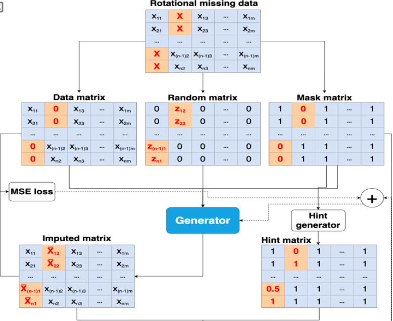
As specified in the PGAIN-VS architecture, there is a random variable with values of {0 , 1} ^d , M = ( M ₁ ...,M _d ), derived from Y, which is the data vector observed by sensor , and M is the mask vector.

We define a new space where ∗ is simply a point that does not belong to any S i . In other words, it is a value at the period of time that a specific location is not equipped with sensor S, with i ∈ {1..., d }. Let is a new random variable and is defined in the following way Eq. (1):

Obviously, M can be recovered from .

The generator, G , in PGAIN-VS takes the three variables with the Pearson correlation (Pc) arrangement, M and noise N as inputs and produces the prediction .

Basically, the random variables are defined and as shown in Eq. (2) and Eq. (3):

where ⊙ is the elementwise multiplication. is the imputed value vector for which the data points are predicted by PGAIN-VS. is the complete data vector obtained by combining the observed data vector in a period of time extracted from the combination of complete and incomplete observation and replacing ∗with the corresponding value of . The noise passed into the generator is (1 − M ) ⊙ because the target distribution is

The discriminator D in PGAIN-VS is considered an adversary for training G to determine the observed or predicted components. D : Y → [0 , 1] ^d with the component D( ) at the i-th position following the probability that the value of at the i-th position is observed by sensor .

PGAIN-VS still uses the “hint” defined in 7 in the process of missing data imputation. and H are accepted as the inputs passed to D . H is formed as follows:

where U ∈ {0 , 1} ^d is defined by uniformly sampling k from {1, 2, ..., d} at random and then setting Eq. (5):

In PGAIN-VS, D is trained to increase the likelihood that it will accurately predict M , and G is trained to decrease the likelihood that D will predict M . The general objective function and loss function are briefly described as Eq. (6) and Eq. (7) below:

In general, the PGAIN-VS algorithm can be expressed in detail by the following pseudocode (pseudocode for the PGAIN-VS algorithm):

Algorithm. Pseudocode of the PGAIN-VS algorithm

Pearson correlation and sensor arrangement calculations

Input : Missing data of sensor Sf and data frame of other sensors Sc

Output : Numpy 2-dimensional array with Pearson arrangement

for i = 0 .n _Sc do

p _i ← Pc ( Sf, Sc _i )

end for

The sc list was rearranged in descending order based on Pearson’s

Convert the Sc data frame to a 2-d numpy array

Begin training of PGAIN-VS

Input : D is the size of batch n _D , G is the size of batch n _G. Output : Imputed data.

Stochastic gradient descent (SGD) is applied.

while until the training loss converges:

(A) Optimize D

Generate n _D samples through , noise and hint

for i = range ( n _D ):

end for

Use SGD to update D.

(B) Optimize G

Generate n _D in the same way as above

for i = range ( n _G ):

end for

Use SGD to update G.

end while

a. Sensor rotational measurement description

In theory, there is always a correlation among collected data, which indicates relationships and similarities among spatial positions. Thus, we define C = ( C ₁ ...,C _d ) as a correlation variable of sensor S _i with the remaining values in the range [0 , 1] ^d and then apply PGAIN-VS to the dataset with its features arranged by Pearson correlation C to obtain imputed values . R = ( R _{S 1} ...,R _Sd ) is defined as a ranking variable calculated with the Borda voting method, and the weight of sensor S _i is determined by R _i . We define a formula to calculate the weight of a single sensor S _i as shown in Eq. (8):

where υ _i is determined by adding the 95th percentile of the absolute errors. Then, the vote is defined as Eq. (9):

where pos _i ( j ) represents the position of sensor j , the total number of sensors used is n _sensors = d , and w _i is the weight calculated.

The whole set of rotational measurement data can be described as follows (Eq. (10)):

Figure 1 . Sensor rotational measurement architecture

where are normal observed values with the i-th rank arranged in descending order from left to right and ∗ are unobserved values during the time when sensor was not present. The number of ∗ on each feature and the number of features having ∗ are determined by solving the optimization mentioned in Eq. (11). Ambitiously, we want to have more ∗ appearing in the dataset, but the reliability of our solution is still preserved.

b. Objective

SRM is considered a black-box optimization (BBO) with constraints, as PGAIN-VS is a machine learning model; thus, there is no analytical form for the objective function. PGAIN-VS is the vector-valued black-box function for the SRM BBO described as f ( x ): X → R ^d , where X is the search space of interest and has the same d -dimension as S defined earlier. Identifying the set of Pareto optimal solutions is the main goal presented in Eq. (11):

such that every advancement in one objective implies a decline in another. We calculate the finite Pareto set P from the observed data to estimate P ^∗ .

In this paper, the PGAIN-VS virtual sensor inspired by GAIN [7] was used as the main mediator to impute missing values. The Borda count 22 method was applied to determine the weight of the sensors before solving the SRM BBO. The SRM BBO is considered the objective optimization method because the minimum RMSE is set as the main objective function, the maximum number of reduced physical sensors is set, and the maximum measurement interval is set.

Mathematically, the equation of the SRM can be written as follows:

where x is the solution, F is the feasible set, f _e is the minimum RMSE objective function, the two others are g _n , the maximum number of physical sensors possibly involving the SRM, and h _i , the maximum observation interval. c ₁ , c ₂ , and c ₃ are the threshold constraints of the functions, and min/max is the combined object operation.

c. Sensor rotational measurement algorithm

The following approach, described in pseudocode, was used to evaluate the ranking supported by Pearson correlation using PGAIN-VS on the 20% of test data that were missing to automatically choose a selection of sensors to be utilized as predictors.

Algorithm. Pseudocode for the sensor ranking

Input : Data of the whole sensors in the list Sl

Output : The rank of the sensors in descending order

foreach sen in Sl do i i← 0

for k = 0 .n _Sl − 1 do

Discarded sensors: S _discarded ← Sl [0: k ]

Remaining sensors: S _remain

remain ← set ( Sl ) − set ( Sdiscarded ) − set ([sen])

error _i ← PGAIN-VS( S _i , S _remain )

Empirical cumulative distribution function at the 95% percentile:

ecdf_95 _i ← ecdf(percentile(95 , error _i ))

end for

i++

end foreach

for i = 0 ..npredicted_ _sensors do

Weight: w _i ← sum ( ecdf 95 , groupby ( predicted_sensor ))

Borda vote for sensors: b _i ← Borda ( n _Sremain , w _i )

end for

As previously noted, the SRM is regarded as a black-box optimization problem; hence, OpenBox, an open-source and general-purpose BBO service, was utilized to resolve this problem. The authors claim that OpenBox implements a wide variety of optimization algorithms to achieve excellent performance in diverse BBO issues and that it is able to select the appropriate algorithms and settings based on the parameters of the incoming assignment. Because it can handle situations where the input space has conditions, there are more parameters in the input space, or there are more trials than hundreds of times, we selected the probabilistic random forest (PRF) 23 to solve the problem in this study.

The top influencing sensors can be selected as candidates for applying SRMs to the data. By being arranged very close to one another, the entire data distribution of datasets can be learned and preserved better. Based on this fact, the algorithm for finding the expected results can be defined by the following SRM pseudocode.

Algorithm. Pseudocode of SRM

Input : Data of the whole sensors, Sl, arranged by the Borda ranking

Output : RMSE, number of SRM sensors and interval

Definition of the configuration space

Add the srm_num and miss_rate variables to the OpenBox space cs

Definition of the RMSE objective function with configuration space cs

( srm_num , miss_rate ) ← cs.get ()

← create_rotation_data ( srm_num, miss_rate )

← PGAIN VS ( )

rmse ← rms_ loss

return objs [ rmse ]

Run OpenBox with the objective

result ← optimizer.run ()

Calculation of results

Min RMSE value: min(results.get( rmse ))

Number of locations: result.get( srm_num )

Interval: result.get( miss_rate ) x interval ₂ adjacent_observation

RESULTS

To evaluate PGAIN-VS, we conducted experiments on the Solar Power (21 sensors) 24 , 25 , Traffic (207 detectors; 50 random sensors were selected) 26 and Rasipihat temperature (12 sensors; 50000 random samples were extracted) 9 datasets, which were also widely used in other works. The details of the datasets are described in Table 1 .

Table 1 Characteristics of the datasets

The answers for the SRM problem are given in Table 2 . We reported the RMSE and R ² values to show the accuracy and reliability of our approach when used to predict missing data with two parameters, the number of reduced sensors and the measurement interval found by OpenBox. We set 100 trials as the maximum number of runs, and the time limit per trial was 180 seconds. A probabilistic random forest was used as the surrogate model for OpenBox to solve the SRM optimization problem.

We extracted the top three feasible results for each experiment corresponding to each dataset with different values of RMSE and R ² , but they were still guaranteed to be within an ideal boundary of approximately 0.10. In addition, to highlight the effectiveness of arranging sensors based on Borda counting, we listed both the ranking and nonranking results for visual comparison. The output shows that the RMSE and R ² obtained using the Borda voting arrangement tend to be significantly better. More importantly, the number of sensors can be reduced, and the time required for a rotation turn seems to increase. This can be clearly observed in the Solar dataset when there is a large distance between the minimum value and the maximum value, as well as for the other parameters described in Table 1 . For the two remaining datasets, especially for Raspihat, we cannot see equivalence because of minor differences in the observed data among positions, but generally, the expectation was still preserved.

Instead of providing the best output for the SRM optimization problem, our approach also yields a few possible results, as shown in Table 2 , from which a suitable choice can be selected depending on the needs of the real circumstances. For example, in the case of the Solar dataset, removing fewer than 4 sensors may be a better selection, but 6 sensors with an RMSE of 0.077 and an R ² of 0.829 should be selected when considering economic considerations (up to an approximately 28% reduction). Similarly, a list of possible combinations was given with up to 5 sensors removed (approximately 45% reduction) for the Raspihat dataset and up to 6 sensors (approximately 12% reduction) for the Traffic dataset. Therefore, depending upon the decision to implement a trade-off strategy, the greater the prediction error accepted is, the more sensors can be saved.

Figure 2 , Figure 3 , Figure 4 show images of the imputed and actual data of the sensors applying the SRM after solving the BOO problem. We can easily realize that the distance between the predicted and observed data is not too large. The imputed data still assure the overall data distribution of the datasets, so the SRM virtual sensing solution is potentially able to produce accurate data. Obviously, the results found in OpenBox for the optimization problem are reliable. We chose the results of each dataset reported in Table 2 with all the sensors involving the SRM to construct the performance graph. Three sensors with imputed data were selected to illustrate the accuracy of the data.

Figure 2 . Performance on the Raspihat dataset for three sensors ; RMSE = 0.032.

Figure 3 . Performance on the Solar Power dataset for three sensors ; RMSE = 0.077

DISCUSSION

The promising results can be explained by the fact that GAN-based approaches are machine learning models in which two neural networks compete with each other to increase the accuracy of their predictions. Hence, arranging the most impactful sensors adjacent helps the data distribution of the whole dataset be learned and preserved better. In addition, as designed, OpenBox is able to recognize the distribution of datasets after several iterations, so it tends to converge at a point; then, the minima of the RMSE are found with different adjustments of the duration and the number of physical sensors to be cut off.

The experimental results affirm the potential benefit for businesses when the number of sensors used in reality can be lower, so the deployment and management costs are surely lower, and the productivity is greater. In addition, the ability of the PGAIN-VS to impute multiple missing-data dimensions was transparently demonstrated through the SRM.

Figure 4 . Performance on the traffic dataset for three sensors ; RMSE = 0.096

More importantly, a new introduction to rotational measurements may lead to more and more ideas for dynamic observation in the future. Nevertheless, our approach is expected to work well with continuous environmental data, so it requires measurements taken on an interval scale. In contrast, the accuracy of these methods may not be guaranteed.

CONCLUSIONS AND FUTURE WORK

In this paper, a novel dynamic sensor rotation measurement approach, SRM, which takes advantage of PGAIN-VS to determine the best subset of physical sensors, was introduced. Various experiments with real-world datasets show that the SRM is capable of finding and replacing real sensors with virtual ones when limitations may arise from its economical or natural nature. The SRM allows dynamic data observation when physical sensors can be moved around positions to perform their jobs. More importantly, SRM provides businesses with a financially beneficial trade-off strategy, as it helps reduce the cost of equipment and the deployment and management of a number of physical sensors to be installed in a spatial area. Finally, the SRM proves the ability of PGAIN-VS to impute multiple missing-data dimensions.

Future work will investigate how to add deeper time series analysis to the solution since it includes temporal information; thus, more valuable information can be extracted and used in the process of training virtual sensors. In addition, for data compression techniques for optimal sensor placement, other correlation metrics should be considered because they help reduce the need for more physical sensors and work with various types of data.

Table 2 The results of SRM solved as black-box optimization by openbox

COMPETING INTERESTS

The authors declare that they have no competing interests.

ACKNOWLEDGEMENT

We acknowledge Ho Chi Minh City University of Technology (HCMUT) and VNU-HCM for supporting this study. We acknowledge the support of time and facilities from the High Performance Computing Laboratory, HCMUT. We also acknowledge the support and collaboration from the TIST Laboratory.

This research was conducted within 58/20-DTDL. The CN-DP Smart Village project was sponsored by the Ministry of Science and Technology of Vietnam.

AUTHORS CONTRIBUTIONS

All authors significantly contributed to this work. All authors read and approved the final version of the manuscript for publication.