Geometry and thermophysical properties of the WAAM wall

Figure 3 (a) shows the baseplate geometry in this study, which is 200 mm in length, 80 mm in width, and 10 mm thick, and its corresponding 3D model geometry. In this study, only the thermal problem was studied. Stainless steel 316 L stainless steel (SS 316 L) was used for both the wall and baseplate materials, and the thermophysical properties were chosen for the numerical simulation, as described in2, 3. As shown in Figure 3(a), the path of the laser encompasses both forward and reverse layers, with one track per layer. This parameter significantly influences the resulting microstructure and mechanical properties of the additive manufactured part 31.

The 3D model, depicted in Figure 3(b), features a six-layered structure specifically designed for this study. To capture areas with high thermal gradients, a refined mesh with dimensions of 0.8x0.1x0.1 mm³ was implemented in three regions: the clad and its immediate vicinities on the substrate. With increasing distance to the deposition path, the element size coarsened toward the edges of the specimen. Based on a convergence study, this mesh size can be evaluated as sufficient, which is consistent with the result reported in 31. As one moves further from the deposition path, the element size gradually increases toward the specimen's edges. A convergence study validated this mesh size as adequate, aligning with findings presented in 31. Additionally, to develop the FE model for thermal simulation, the thermophysical properties of SS316L reported in31 and Goldak’s heat source model (Figure 4) were chosen for the numerical simulations.

In this study, we assumed identical thermophysical properties for both the base plate and the thin wall, despite their differing microstructures. Additionally, we understand that the entire process, including the behavior of the wall geometry, is of paramount importance. While this assumption may appear simplified, it aligns with previous studies in the field31. Nevertheless, it is important to note that this assumption may introduce certain simplifications in the model. Future work could explore the implications of considering distinct thermophysical properties for base plates and thin walls, which may lead to a more comprehensive understanding of the process.

Heat input modeling

A Goldak volume heat source32 based on double ellipsoidal power density distributions was used in this study. Figure 4 illustrates the heat distribution of a double ellipsoidal heat source model. The heat flux is modeled in Z-direction with its parameters were selected as those in 32: a = 7 mm,a = 13 mm, b = 4 mm, c =4 mm,f = 0.6, and f = 1.4.

The WAAM process simulation was performed using ANSYS software. Before the simulation, all the clad layers are considered inactive (dead) elements since they do not exist before the WAAM process (phase prestep). During the process, the dead elements are reactivated successively under the effect of the welding torch using an activation time that was modeled through the welding speed. This method suffers from a computational time disadvantage, but it can help to model the process in practice accurately.

In general, the temperature evolution can be predicted as

where q = [x, y, z, t, m] is a multidimensional vector of the spatial coordinates (x,y,z), the time (t), and the other input parameters (m), i.e., the current intensity. As discussed in the introduction section, solving the above equation is time-consuming, i.e., six hours for one simulation. As a result, we constructed an ML-based surrogate model to reduce computational costs. The following section introduces the specific ML-based surrogate models employed in this study.

ML-based surrogate model

Model selection

Several algorithms, including linear regression, random forest, and feedforward neural networks (FFNNs), can be used to construct ML-based surrogate models. In this study, we choose the FFNN architecture owing to its ability to approximate highly nonlinear relationships within the physics of WAAM. Moreover, the FFNN will be expanded to incorporate an explainable method, thereby enhancing the interpretability of the sensitivity analysis.

Data collection

The training data for the ML model are generated through simulations using the FE model outlined in Sec. 2. These simulations consist of various values of key WAAM process parameters, namely, the current intensity () and velocity (). The resulting training dataset includes four distinct simulations, detailed in Table 1. Each of these FE simulations results in a temperature field corresponding to a specific combination of and .

In each FE simulation, we accumulate a substantial dataset, with a total of 19,126,800 data points (10626 nodes × 1800 timesteps = 19,126,800) for a given pair of U and I. As demonstrated in Table 1, we employ four FE simulations with {I, U} = {120, 0.2}, {126, 0.3}, {138, 0.5}, and {144, 0.6} to train the ML model, yielding approximately 76,507,200 data points. These training datasets are subsequently partitioned into two sets, one for training and the other for validation, allowing for fine-tuning of the ML model's performance.

To assess the predictive accuracy, we subject the ML model to an unseen FE simulation for {I, U} = {132, 0.4} as our testing dataset. This evaluation ensures the robustness and reliability of our model's prediction capabilities.

In addition to improving the prediction accuracy of the model, we added four additional features, namely, the heat source position x, z and the distance from the heat source to the FE nodes d, d. Note that these features are chosen by the trial-and-error approach. To avoid adding substantial length to the paper, the overall description of these features and the feature selection process can be found in6.

In general, the ML model can be represented as

where W is the weight and q is the input, which includes the spatial coordinates (x, y, z), the time (t), the current intensity (I), the velocity (U), the heat source position , and the distance from the heat source to the FE nodes (d, d). The output is the temperature at each spatial coordinate at a specific time.

Explainable ML method

To provide a deeper understanding of the predictive capability of the FFNN-based surrogate model g, we subsequently describe the explanatory ability of the FFNN-based model. In this work, the SHAP method 33, 34 is used to explain the FFNN-based surrogate model. The SHAP method was developed based on Shapley from cooperative game theory 35.

Let N be the set of all input features of the FFNN g, and S denotes a subset of N. The SHAP value assigns a value ϕ (q), with i = 1,2,…,n, to each feature representing this feature's contribution to the model prediction. This value is computed as

where |N| is the number of features in the set N and |S| is the number of features in the set S. However, the SHAP method requires training the model g for all subsets S ⊆ N and thus significantly increases the computational cost. Additionally, most of the ML-based models do not accept arbitrary patterns of missing input. Therefore, the SHAP method was developed to overcome these problems. In particular, the SHAP method proposed an approximation based on conditional expectation as

where q and z are |S|-dimensional vectors that collect values of the features in S from vectors q and z, respectively. As a consequence, the missing features q in Eq. (1) can be randomly drawn from the background data (normally the mean value) to obtain an approximation for g (S). Therefore, the SHAP method significantly decreases the computational cost compared with the original Shapley method. The SHAP method ranks the importance of features on the task performance of the ML model.

Finite element results

Figure 5 depicts the temperature evolution at the middle point of the first layer in the clad, as obtained from the finite element (FE) model in this study. The temperature shows an oscillation behavior named as temperature oscillations that strongly influences the final microstructure. Additionally, after six thermal cycles, the temperature peak exhibits a progressive decrease. This can be attributed to the phenomenon of heat accumulation during the wire and arc additive manufacturing (WAAM) process. It is noteworthy that the number of temperature peaks in the thermal cycle corresponds to the number of layers deposited in the clad. Note that our ongoing experiments are aimed at validating the results obtained from the finite element model. Additionally, we would like to acknowledge that, in the FE simulation, we treated the wall height as a constant, and this can be considered an assumption. It is important to consider how altering the current intensity or laser velocity often leads to variations in wall height. Thus, we will consider this assumption in our future study.

Machine learning-based surrogate model results

This section presents the results of the temperature field prediction by the FFNN-based surrogate model, as discussed in Sec. 3.

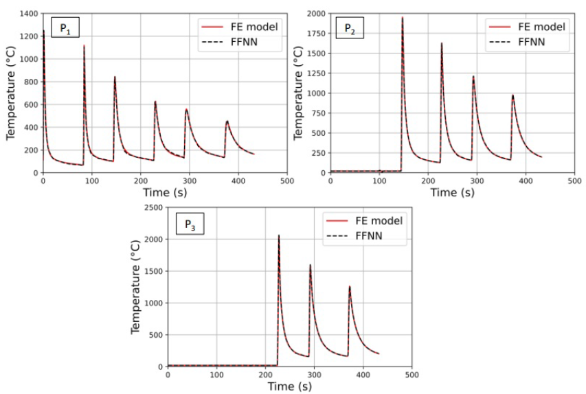
For ease of visualization, we selected three specific points to showcase the temperature evolution. These points are situated in the middle of the first, second, and third layers in the clad, denoted as P1, P2, and P3, respectively, as depicted in Figure 6. It is worth noting that these points are anticipated to demonstrate the most intricate thermal cycles during the WAAM process, characterized by high-temperature peaks followed by gradual cooling cycles, as illustrated in Figure 5. Furthermore, these points were extracted from a distinct test dataset that the model had never encountered during its training and validation phases.

Figure 7 displays the temperature evolutions derived from both the FE model and the FFNN-based surrogate models for three specified points, namely, P1, P2, and P3. The FFNN-based surrogate model accurately captures the thermal cycles at these points, reproducing both the temperature peaks and the subsequent cooling phases. Specifically, the values 36, 37 calculated for these three points exceeded 0.99.

In essence, the FFNN-based surrogate model demonstrates good accuracy in predicting temperature evolution. The subsequent section will discuss the explanation of the FFNN-based surrogate model, employing the SHAP method discussed in Sec. 3. Hereafter, we carry out the discussion section to determine the physics inside WAAM using the ML explainable method.

Sensitivity analysis of the process parameters

The sensitivity analysis of the temperature evolution in response to variations in the current intensity and velocity is depicted in Figure 8. As anticipated, increasing the current intensity facilitates more efficient heat propagation within the printed component, augmenting the energy delivered to the laser and consequently elevating the temperature. Conversely, a reduction in velocity leads to an increase in temperature. This phenomenon can be attributed to the fact that higher scanning speeds entail reduced time spent by the laser at any specific point on the powder bed. Consequently, the energy transferred to the material diminishes, resulting in lower temperatures compared to those of the case with slower scanning speeds.

Sensitivity analysis of the ML-based surrogate model

Figure 9 shows the 95% quantile SHAP values corresponding to each feature. The absolute SHAP value is a measure of the feature contribution to the difference between the predicted temperature and its average value. Note that the 95% quantile is chosen since it is a standard evaluation criterion in statistics. As observed in Figure 9, ,and constitute the most influential additional features for temperature prediction. In contrast, other features, such as x, y, z, t, U, and I, play a minor role in temperature prediction. Note that these features are basic features; therefore, they should not be translated as negligible parameters.

Using the SHAP analysis information in Figure 9, this section introduces one base and four reduced FFNN-based models, resulting in five models to verify the ranking of the feature importance for temperature prediction and to determine the relevant features contributing to the temperature evolution behavior. The base model consists of only six basic features. The five consecutive reduced FFNN-based models are built by adding each feature in the order of their 95% quantile SHAP values. The description and values of the five FFNN-based models are included in Table 2.

As listed in Table 2, the base model poorly predicts the temperature fields, with a low R2 value of 0.7211. In addition, the R values of each reduced model increase gradually with the addition of each feature. The R value of the FFNN-based model reached 0.9964 for all the features. This result confirms that d plays a vital role in temperature prediction.

Computational cost assessment

Table 3 illustrates the computational cost incurred when employing both the FFNN-based and FE models for temperature field prediction. As depicted, the FFNN-based model achieves this task in approximately 20 seconds, a substantial reduction of 3272 times compared to that of the FE model, which requires 18 hours. In summary, utilizing the FFNN model significantly speeds up the optimization and uncertainty quantification process, especially when thousands to millions of temperature field predictions for varying process parameters are needed.