New model for low-end computers: ResNet and VGG-16

Abstract

ResNet-50 is a powerful architecture of convolutional neural networks, which gives truly high accuracy and very small error rate. However, this architecture seems not to be very effective when executing in low-end computers because of the small batch size for satisfying limited resources, which is not good for batch normalization. There is also an attempt to use VGG-16 as an alternative method, but vanishing gradients occur often. The proposed model is an improvement of VGG-16 using ResNet for shortcuts to prevent vanishing gradients, and the new architecture does not require batch normalization. As a result, the proposed model achieves a high test accuracy of 85.4%, while ResNet-50 achieves a test accuracy of 75.9% after 40 epochs of training 14,034 images from the Natural Scenes from Image Classification Challenge by Intel. This model is effective for applications related to image processing.

INTRODUCTION

Computer vision is a field that helps obtain meaningful information from visual data such as images, videos or other visual sources 1 . Computer Vision includes common tasks such as Object Detection, Image Segmentation, Image-to-Image Translation, etc. Deep learning is considered a breakthrough in solving computer vision problems. The development of deep learning has led to the explosion of many applications that bring high efficiency to computer vision tasks, especially the emergence of convolutional neural networks (CNNs).

In recent years, many CNN architectures have been created to improve the performance of computer vision tasks, especially in image classification. All the architectures have convolutional layers to help extract image features from the image input. Common architectures for image classification are VGG-16, VGG-19, ResNet, DenseNet, LeNet, AlexNet, Inception (GoogLeNet), and ResNeXt. Among these architectures, residual networks 2 are extremely important because they allow people to extend the layers of models deeper without the negative effect of vanishing gradients. ResNet has many variants, such as ResNet-18, ResNet-34, ResNet-50, and ResNet-152. ResNet can train the images with a truly high accuracy. However, it seems to be less effective when running on low-end computers. With low-end computers, the memory is limited, and the batch size must be small to avoid resource exhaustion errors when training. The small batch size can affect the training results, such as increasing the error values.

The main contribution of the paper is to suggest an alternative model to solve the problems for low-end machines by:

• Analyzing the problems of the traditional model for low-end computers.

• Proposing an improved model and showing the results of the implementation.

Following this introduction, the paper presents six contents: problem statements, proposed model, dataset, experimental results, discussion and conclusion.

PROBLEM STATEMENTS

ResNet-50 3 is an effective model for image classification tasks with very high accuracy and a very low error rate compared to many models. However, ResNet-50 becomes ineffective with low-end computers. The large number of parameters due to deep networks could be a major problem for limited memory. Some machines have resource exhaustion errors when attempting to train large batch sizes of images by some models with large parameters, such as ResNet-50. The problem is how to build a model for low-end computers.

The temporary solution is to decrease the batch size, but the accuracy is quite low because of batch normalization 4 , which is not good for small batch sizes. An alternative that could be considered is the modified version of VGG-16 5 by reducing some units at the fully connected layer. Another problem is the vanishing gradient, when the accuracy almost does not improve after many epochs pass.

Batch normalization

Batch normalization is a method to standardize the inputs for each mini-batch. Batch normalization helps the training faster and stabilizes the distribution of inputs during training. However, batch normalization works well with a large batch size.

In Rethinking "Batch" in BatchNorm research conducted by Facebook AI Research 6 , batch size is closely related to the error of the training using batch normalization, as shown in the Figure 1 . The smaller the batch size is, the larger the error value of the training result. The low-end machines can only afford a small batch size of 16, 8 or smaller, or our machine satisfies roughly the batch size of 16.

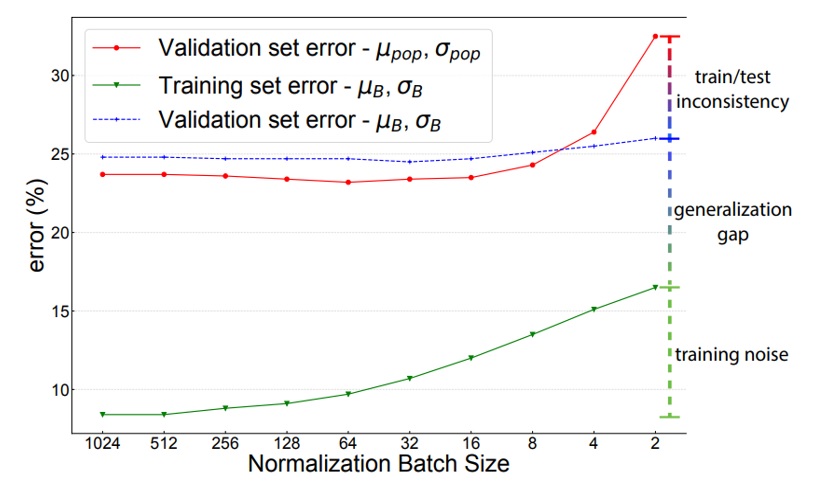
Figure 1 . Batch Size and Batch Normalization 7

7" width="300" height="200">

Vanishing gradient

Another method to avoid the use of batch normalization is using VGG-16. However, in some cases, the training accuracy after a significant number of epochs almost does not improve. The reason for this problem is the vanishing gradient 8 . The number of layers of VGG-16 is much less than that of ResNet-50, but without skip connections, VGG-16 still has the possibility of leading to a vanishing gradient.

A vanishing gradient occurs when there are many layers in the network. In the backpropagation process, the weights change to minimize the loss. With a vanishing gradient, the value of the product of derivatives that determine the change in weights and biases is close to zero. Therefore, the weights almost do not update, and the network does not learn anymore. As a result, the training accuracies at every epoch are nearly the same.

PROPOSED MODEL

Proposed Model Architecture

CNNs have many architectures that can be used to solve different types of problems. All the architectures have convolutional layers to help obtain image features from the image input. Common architectures for image classification are VGG-16, ResNet, DenseNet, LeNet, AlexNet, Inception (GoogLeNet), and ResNeXt. In addition, YOLO (You Only Look Once) is a very popular choice to solve object detection problems. In image segmentation problems, U-net, PSPNet and SegNet are also widely used.

The proposed model architecture is an improvement of VGG-16 by using a residual network. The VGG-16 originally has 16 layers as 13 convolutional layers and 3 fully connected layers. In the proposed model, a small change has been made in the fully connected layers. We reduce the units in each fully connected layer because of the limitations of our computer. With the residual network applied, this model can avoid the vanishing gradient. The residual network can solve the problem by using skip connections (shortcuts). The skip connection helps connect a layer to another further layer, skipping some layers in between. The skip connection model is shown in the Figure 2 .

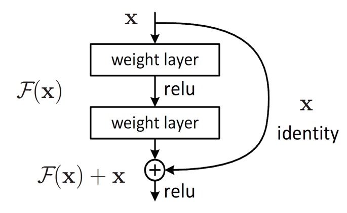
Figure 2 . Skip connection in ResNet 2

2" width="300" height="200">

Residual Network

A residual network (ResNet) is a type of deep neural network architecture designed to overcome the problem of vanishing gradients, one of the difficulties causing the training process to converge very slowly or even become stuck. The gradients have to flow through many layers to update the weights at the earlier layers, so the vanishing gradient often occurs in networks with a large number of layers.

ResNets allow the creation of much deeper networks compared to traditional neural networks without encountering the vanishing gradient. The basic idea of the solution is to add skip connections or shortcuts between layers. The shortcuts help the gradients flow more easily through the network. Therefore, the residual network is considered an innovative solution in making it possible to create deep networks with a large number of layers for better training accuracy.

The proposed model uses shortcuts for each group of convolutional layers. An extra convolutional layer with a kernel size of 1x1 is inserted into each shortcut to make the output dimensions from the skip connection identical to the output dimensions from the main path. The input image of the model has dimensions of 224x224x3, where the image height is 224, the image width is 224, and 3 means the image is in RGB with 3 channels (red, green, blue). The proposed model architecture is shown in Figure 3 .

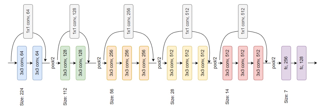
Figure 3 . ResNet + VGG16 architecture

Network Parameters

The parameters of the proposed model are shown in Table 1 .

Table 1 Proposed model parameters

Convolutional Neural Network Layers

Convolutional Layer

The convolutional layer is the most important layer in convolutional neural network layers. It is the first layer that extracts the features from the images. Image features are necessary information such as edges or sets of points to represent the content of the image. The layer consists of filters or kernels, which have dimensions of 3x3. The images that go through the convolutional layer will be processed by the convolution operation with the filters. The filters slide over the areas of the input images, and they take the dot product with the area that is slid. The principle of the convolution operation is shown in Figure 4 .

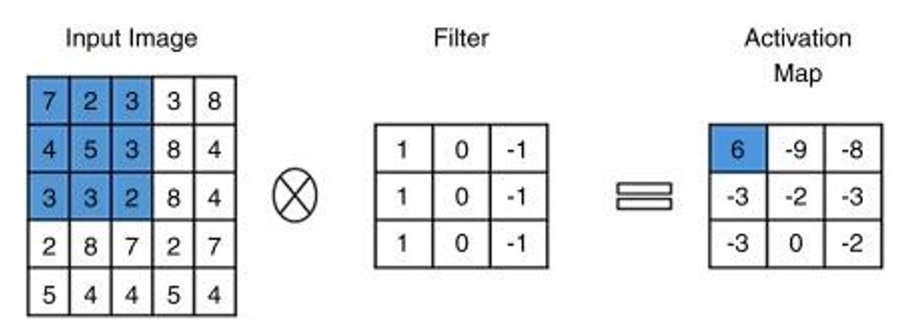
Figure 4 . Convolution operation 9

9" width="300" height="200">

The output of the convolution operation between each kernel and an image is the activation map (or feature map), which is also a matrix containing the feature of the image. The dimensions of the feature map are shown in (1).

Feature map dimensions = (h – f _h + 1) x (w – f _w + 1) x 1 (1)

where

Filter dimensions = f _h x f _w x d

Input image dimensions = h x w x d

h: input image height,

w: input image width

d: input image depth

f _h : filter height

f _w : filter width

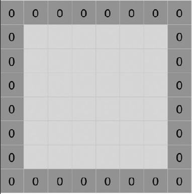
Information at the edge of the images may be neglected or the dimensions of the output decrease when the size of the filters is larger than 1x1. Therefore, we use zero-padding, or padding ='same', to insert the zero values into the boundaries of the image input to prevent the problems above. An input image after adding one layer of zero around the edges is shown in Figure 5 .

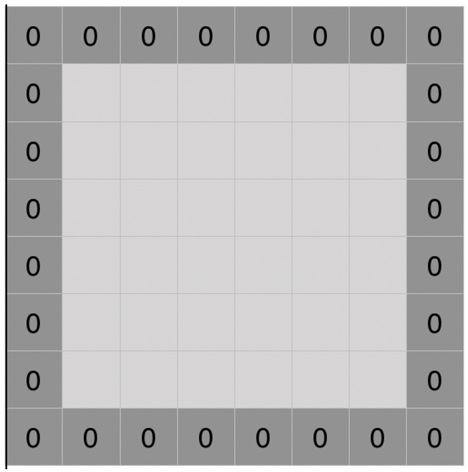
Figure 5 . Zero-padding added to an image 10

10" width="300" height="200">

The padding length will vary depending on the size of the filters. The formula of the padding ='same' is shown in (2).

p = (kernel size -1)/2 (2)

where

filter size = filter height x filter width

padding height = (filter height -1)/2

padding width = (filter width -1)/2

Pooling Layer

The pooling layer, which is usually inserted between the convolutional layers, is used to reduce the size of the feature map so that the computational costs decrease. The feature map after going through the pooling layer still holds the important properties of the images. This layer summarizes the features in the areas of the feature map.

The dimensions of the feature map after going through the pooling layer are shown in (3).

Feature map dimensions = (h – f _h + 1)/s x (w – f _w + 1)/s x d (3)

where

Input (old feature map) dimensions = h x w x d; Pooling filter dimensions = f _h x f _w ; Stride length: s

h: Input (old feature map) height

w: Input (old feature map) width

d: Input (old feature map) depth

f _h : filter height

f _w : filter width

s: Stride length

Max pooling and average pooling are common types of pooling operations. We choose max pooling for use in the proposed model. This operation chooses the maximum element from the area of the feature map with the specified pooling filter size. The operation is shown in Figure 6 .

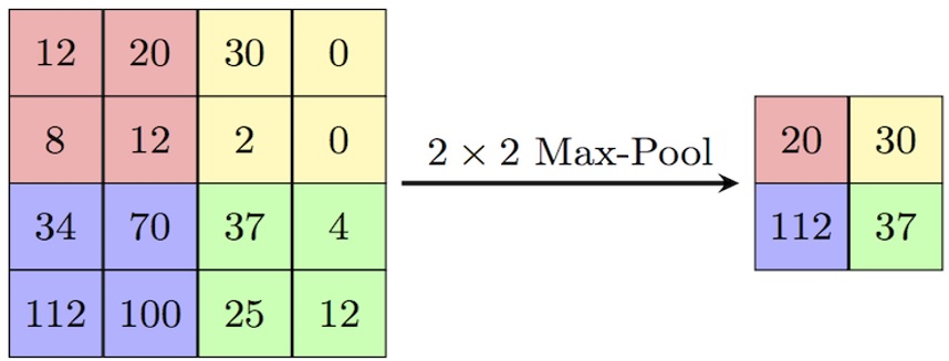
Figure 6 . Pooling layer with size 2x2 11

11" width="300" height="200">

Fully Connected Layer

The fully connected layers consist of many neurons connected to the neurons in the next layer, as shown in Figure 7 .

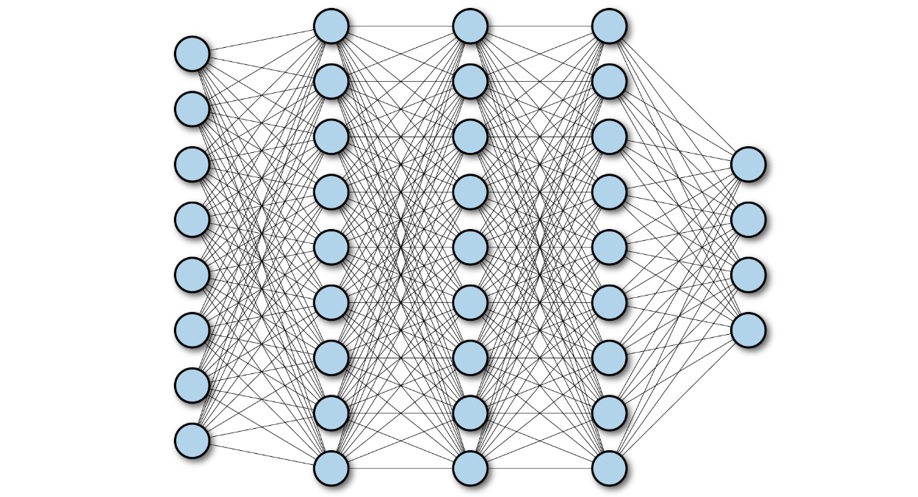
Figure 7 . Fully Connected Layers 12

12" width="300" height="200">

An output feature map from the previous layer, which is in matrix representation, is converted into a vector. Then, the vector will be the input of the fully connected layer. The classification process is performed at the fully connected layers. In these layers, ReLU has been used as an activation function (not in the output layer). The function returns maximum input if it is positive or 0 if the input is negative. The ReLU function has simple mathematical operations, so it makes the calculation faster than using sigmoid and tanh.

Finally, the output goes into the last layer called the output layer. This layer gives the desired predictions through the activation function. The common activation functions of the output layer are Softmax, Sigmoid, and Linear. The proposed model uses the softmax function as the activation function for the output layer, which is specifically used for multiclass classification tasks. The Softmax function returns the probability of each class.

Softmax function

The Softmax function is a mathematical function mapping a vector of real numbers to a probability distribution by transforming the input values into probabilities that have a total of 1.

The softmax function is often used as the last layer of a neural network, where the input to the function is a vector of activations from the previous layer and the output is a set of class probabilities. The higher the probability value of the class is, the higher the probability that the input data belong to that class.

The formula for the softmax function is shown in (4) as follows:

: The input vector containing

i: The index i in the input vector

: The value at the index i in the input vector

k: The last index in the input vector

DATASET

The dataset is about natural scenes around the world. These data were first published on the website https://datahack.analyticsvidhya.com to host an Image Classification Challenge by Intel 13 . The dataset is downloaded from Kaggle. The dataset includes 17,034 images of 14,034 images used for training (~81%), 1,580 images used for validation (~10%) and 1,420 images used for testing (~9%). All the images are divided into 6 classes: buildings, forest, glacier, mountain, sea, and street.

In addition, two other datasets of “flowers” 14 and “dogs and cats” 15 are used.

The flowers dataset includes 3,670 images with 2,934 images used for training (~80%), 364 images used for validation (~10%) and 372 images used for testing (~10%). All the images are divided into 5 classes: daisy, dandelion, roses, sunflowers, and tulips.

The dataset includes 24,998 images with 19,644 images used for training (~80%), 2,463 images used for validation (~10%) and 2,891 images used for testing (~10%). All the images are divided into 2 classes: dog and cat.

To increase the number of images in the dataset and reduce overfitting, data augmentation techniques 16 are performed. We use the API of TensorFlow, which is ImageDataGenerator, to support increasing the diversity of the dataset. The original images are changed by rotating, shifting horizontally and vertically, shearing, zooming and flipping.

EXPERIMENTAL RESULTS

Training

The experiment is executed on an ASUS laptop with an AMD Ryzen 7 4800H CPU @ 2.90 GHz, NVIDIA GeForce GTX 1650 Ti GPU and 8 GB RAM. The batch size of training is set to 16 due to the memory limit of the GPU and RAM.

The proposed model and ResNet-50 are trained for 40 epochs for comparison with each other in terms of training accuracy, validation accuracy, training loss and validation loss. Both models are optimized by the Adam optimization algorithm with the initial learning rate set to 0.001. Sparse Categorical Cross-entropy is chosen as the loss function for both models.

Results

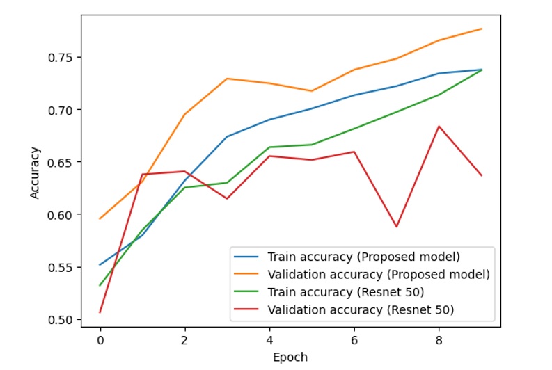
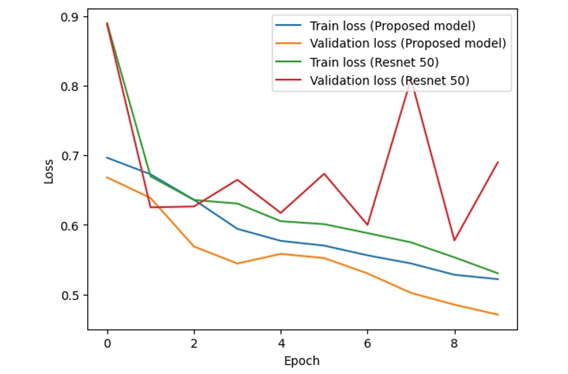
The proposed model gives 86.1% accuracy and 0.37 loss on the training set and 85.4% accuracy and 0.39 loss on the test set, while the ResNet-50 model produces a training accuracy of 86.4%, a training loss of 0.38, a test accuracy of 75.9%, and a test loss of 0.73. Figure 8 and Figure 9 show the training accuracy, training loss, validation accuracy, and validation loss of the proposed model and ResNet-50 through 40 epochs.

In addition, some other results on the flower dataset and dog and cat dataset are also shown in Figure 10 , Figure 11 , Figure 12 and Figure 13 .

Figure 8 . Training and validation accuracy of the proposed model and ResNet-50

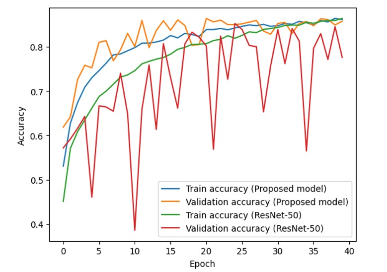
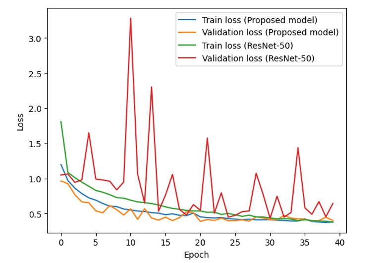
Figure 9 . Training and validation loss of the proposed model and ResNet-50

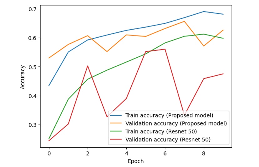
Figure 10 . Training and validation accuracy of the proposed model and ResNet-50 (flowers dataset)

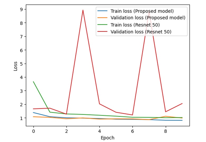
Figure 11 . Training and validation losses of the proposed model and ResNet-50 (flowers dataset)

Figure 12 . Training and validation accuracy of the proposed model and ResNet-50 (dogs and cats dataset)

Figure 13 . Training and validation loss of the proposed model and ResNet-50 (dogs and cats dataset)

DISCUSSION

From the above figures, it is clear that with the combined model of ResNet and VGG-16, the difference between the training accuracy (the blue line) and validation accuracy (the orange line) is relatively stable and small, while the difference between the training accuracy (the green line) and validation accuracy (the red line) fluctuates with unstable amplitude. This is the same as the difference between the training loss and validation loss in the two models.

If we consider and analyze the accuracy in Figure 8 , Figure 10 and Figure 12 , the accuracy (both training accuracy and validation accuracy) from the suggested model is higher than the accuracy from the traditional ResNet. In terms of loss in Figure 9 , Figure 11 and Figure 13 , the loss from the suggested model is lower than the loss from the traditional ResNet.

Based on the experimental results of two models on the dataset, the proposed model works better than ResNet-50 with higher accuracy and lower loss. The accuracy and loss of the proposed model are more stable than those of ResNet-50.

CONCLUSION

This paper proposes a new model using ResNet in a modified VGG-16 architecture to satisfy the strict requirements of low-end machines. ResNet-50 is not very effective with a small batch size because of batch normalization. The new model is based on the VGG-16 architecture, which does not need BatchNorm layers. The original VGG-16 model has very large units at the fully connected layers, which can exceed the limit memory when performing calculations. Additionally, the VGG-16 model reveals a new challenge, the vanishing gradient. Therefore, we add ResNet for VGG-16 and reduce the units to solve the problem. The experimental results show that the proposed model has higher accuracy and lower loss than ResNet-50 in the training set, validation set and test set. The test accuracy of the proposed model is 85.4%, while that of ResNet-50 is 75.9%. Therefore, in the condition of limited memory for low-end computers with a small batch size, the proposed model has better performance than ResNet-50. With this result, the proposed model can be used to replace former ResNet models for applications run on low-end computers. The implementation of this proposed model to solve the problems of object classification and image assessment is our next research direction.

LIST OF ABBREVIATIONS

CNN - Convolutional neural networks.

ResNet - Residual neural network.

VGG - Visual Geometry Group (VGG-16 was proposed by Karen Simonyan and Andrew Zisserman of the Visual Geometry Group Lab of Oxford University in 2014).

ACKNOWLEDGEMENT

We thank the AIoT group of the School of Computer Science and Engineering for giving me the motivation to complete the model with the expected effectiveness.

CONFLICT OF INTEREST

The authors declare that they have no competing interests.

AUTHOR’S CONTRIBUTIONS

Hoang Linh Nguyen built and implemented the model, and analyzed the results.

Kha Tu Huynh proposed idea, supervied the implementation, evaluated the efficiency of the model, wrote the paper, reviewed and revised the paper.